Volume Analysis🙏🏻 (signed) Volume Analysis is 2 of 2 structural layer / ordeflow analysis scripts, while the first one is Liquidity Analysis. Both are independent so can’t be released together as a single script, but should be used together.
The same math used in this script can be applied to other types of aggressive volume data: non-aggregated flow of market orders, volume traded of put vs call options.
There’s no universal agreement about terminology, but this script works with volumes signed by the aggressor who initiated a transaction. Then these volumes get aggregated by time and a cumulative sum is calculated. Mostly this is widely known as Cumulative Volume Delta.
However this script works with 'inferred' volumes vs the provided ones. It’s the better choice for equities, bonds; neutral choice for currencies; and suboptimal choice for natural and artificial commodities.
Contents:
Output description;
How to analyze & use the outputs;
How to use it together with Liquidity Analysis script;
How did I use both scripts to finish The Leap profitably and skipped many losses.
1. Output description
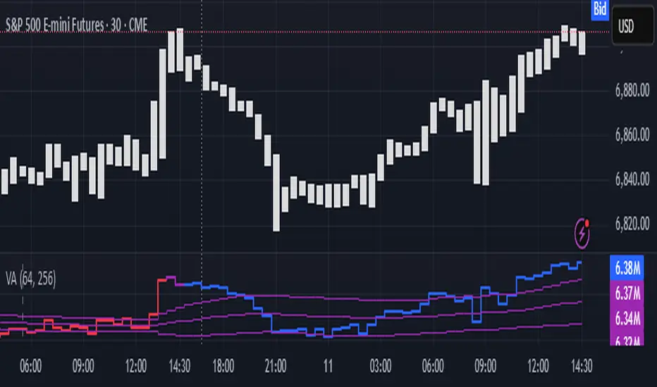
Color of the CVD line reflects (signed) volume imbalance state: red is negative, purple is neutral, blue is positive.
3 purple lines are lower deviation (lower band), basis (middle band), upper deviation (upper band): used to generate signals by a ruleset that would be explained in a minute
Gray number in the script’s status line is the advised input you may put into Inferred volume multiplier in script’s setting, I will explain it
Vertical dash line marks the moving window end, this way you can be certain over what exact data you see the profile was built.
2. How to analyze & use the outputs
Setup up the script:
Moving window length: set it to ~ ¼ of your data analysis window. E.g if you see on your charts and use ~ 256 bars, set the length to 64.
Inferred volume multiplier: you can easily leave it 256, this is not a critical factor for the math, it’s mostly there if you want to ~ equate inferred volumes with real ones in scale. For this, use the gray number in the script status line, it’s calculated as ratio of long term real volumes weighted avg to long term inferred volumes weighted avg.
Again, changing the inferred volume multiplier won’t affect the math.
Use 2 timeframes: main one and a far lower one 3 steps down, just like on the screenshot.
Find out current volume imbalance state:
As mentioned before, based on CVD line color, it can be negative, neutral or positive. This is the state variable that changes slowly and denies/confirms the signals generated by crossovers of CVD line and 3 purple thresholds.
For this I use my own very fast and lightweight metric that is totally statistically grounded, utilizes temporal information, and calculates volume imbalance without using heavy math like regressions as it’s usually done. It also provides a natural neutral zone, when volume imbalance is not strong enough to be confirmed.
...
CVD-based signals:
First you need to understand what precisely a touch of a threshold is:
Touch: an event when either of these 2 happens:
One CVD datapoint is above the threshold, and the next CVD datapoint is below the threshold
One CVD datapoint is below the threshold, and the next CVD datapoint is above the threshold
These are usually called crossovers/crossunders.
Now with the 3 purple thresholds we follow this logic:
Monitor the last touched threshold;
Once another threshold is touched, here we may generate a signal but only once !, after the first generated signal at that threshold we can’t generate more signals on this threshold, we need to wait when CVD comes to another threshold.
If CVD touches one threshold, and then goes down and touches another threshold downwards, we wait when CVD makes a datapoint above this threshold. When it happens, we register a long signal
If CVD touches one threshold, and then goes up and touches another threshold upwards, we wait when CVD makes a datapoint below this threshold. When it happens, we register a short signal
However, don’t open new trades against the current volume imbalance state. So don’t open shorts when the CDV line is blue, and don’t open longs when CVD line is red.
Btw, this technique I call it “reclaim” of a level/threshold. It can be applied to horizontal levels, and it’s very powerful especially when you fade levels on very volatility assets like BTC. This technique allows you to Not fade a level straight away, but wait when price goes past the level a bit, and then comes back and reclaims it, only there you enter, and moreover you now have a very well defined risk point.
The last part is multi-timeframe logic. Prefer to act when a lower timeframe is Not against the main timeframe. That’s all, no multiple higher timeframes are needed.
3. How to use it together with Liquidity Analysis script.
That script also has a mean to generate its own signals, and another state variable called Liquidity Imbalance.
So now you’re not only looking at volume imbalance but also at liquidity imbalance that would deny/confirm the CVD based signal. You need at least one of these two to favor your long or short.
This is the same logic widely used in HFT, where MM bots cancel/shift/resize orders when book is too onesided And ordeflow is one sided as well.
4. How did I use both scripts to finish The Leap profitably and skipped many losses.
Even tho you can use structural information as your main strategic layer, as many so-called orderflow traders do, I traded in objective style: my fade signals were volatility based in essence, and I used ordeflow for better entries and stops, but most importantly to skip losses.
When ‘both‘ liquidity imbalance and volume imbalance (in their main timeframes) were against my trades, I skipped them all, saving many ~$500 stop losses (that was my basis risk unit for the Leap). Unless I had a very strong objective signal, i.e. confluence of several signals, or just one higher timeframe signal, I did all these skips.
I traded ~ intraweek timeframe, so I was analyzing either the last 230 30min bars or 1380 5min bars. Both Liquidity Analysis and (signed) Volume Analysis scripts were set to moving window length 46 or 276 for either granularity.
I finished the leap with 9% profit and max DD ~ 5%, a bit short of my goal of 12.5%. If not these 2 scripts I would’ve finished a bit above breakeven I think.
,,,
Another thing, I made these 2 scripts invite-only because they are made particularly for trading, particularly for certain types of market data. These are tools adapted for particular use case, not like my other posts with general math entities like Kernel Density Estimation or Kalman filter, that you can take and apply properly on any data you need yourself.
However these are made from general math entities like everything else. ‘All’ the components are available in my other scripts, ideas, and other sources related to me. If you want to reverse-engineer these, you can find all the components you need in my already posted open source work.
∞
Orderflow
Liquidity Analysis🙏🏻 Liquidity Analysis is 1 of 2 structural layer / orderflow layer analysis scripts. Both are independent so can’t be released together as a single script, but should be used together. The second one which is called (Signed) Volume Analysis is incoming.
The same math used in this script can be applied on other types of profile-like data: orderbooks, trading volumes of all options for each strike.
Important: market or volume profile, just as orderbooks and options traded volume by strikes, are all liquidity ‘estimates’, showing where liquidity is more likely or less likely to be. These estimates however, especially combined with other info, are really useful and reliable.
This script works with inferred volumes vs the provided one. It's the better choice for equities, bonds; neutral choice for currencies; and suboptimal choice for natural & artificial commodities.
Contents:
Output description;
How to analyze & use the outputs;
How to use it together with upcoming (Signed) Volume Analysis script;
How did I use both scripts to finish The Leap profitably and skipped many losses.
1. Output description
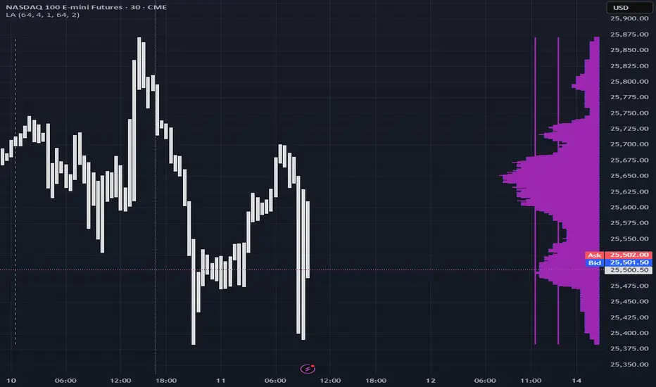
Color of the profile reflects the liquidity imbalance state: red is negative, purple is neutral, blue is positive.
Bar coloring represents history values of liquidity imbalance for backtesting purposes. It can be turned on/off in the script's Style settings.
Two purple vertical lines represent calculated borders of excessive liquidity (HVN), scarce liquidity (LVN), and sufficient liquidity (NVN) zones.
Vertical dash line marks the moving window end, this way you can be certain over what exact data you see the profile was built.
2. How to analyze & use the outputs
Setup up the script:
Moving window length: set it to ~ ¼ of your data analysis window. E.g if you see on your charts and use ~ 256 bars, set the length to 64.
Native tick size multiplier: leave it at 0 to calculate optimal number of rows automatically, or set it manually to match native tick size multiples you desire.
Use 2 timeframes: main one and a far lower one 3 steps down, just like on the screenshot.
Native lot size multiplier allows to round profile rows themselves to nearest multiples of native lot size. I added this just in case any1 needs it.
Find out current liquidity imbalance state:
As mentioned before, based on profile color, it can be negative, neutral or positive. This is the state variable that changes slowly and denies/confirms the signals that would be explained in the minute.
I use my own statistically grounded imbalance metric (no hardcoded/learned thresholds), that unlike mainstream imbalance metrics (e.g orderbook imbalance as sum of bids vs sum of asks) provides a natural neutral zone, when liquidity imbalance is ofc there but not strong enough to be considered.
…
Profile-based signals: look at profile shape vs 2 vertical purple lines.
where profile rows exceed the left purple line, these prices are considered HVN. Too much potential liquidity is there.
where profile rows don’t exceed the right purple line, these prices are considered LVN. Potential thin/lack of liquidity is expected there.
where profile rows are in between these 2 purple lines, these are NVN, or neutral liquidity zones.
Trading ruleset itself is based on couple of simple rules:
Only! Use limit orders hence provide liquidity in LVNs and Only! use stop-market orders hence consume liquidity in HVNs;
These orders should be put in advance ‘only’. This is how you discover the direction or orders: you can only put sell limit orders above you and buy limit orders below you, and you can only put buy stop orders above you, and sell stop orders below you.
This is really it. It may look weird, but once you just try to follow these 2 rules letter by letter for 1 hour, you’ll see how liquidity trading works.
Now once you know that, just don’t open new trades against the liquidity imbalance state. So don’t open shorts when the profile is blue, and don’t open longs when it’s red.
The last part is multi-timeframe logic. Prefer to act when a lower timeframe is Not against the main timeframe. That’s all, no multiple higher timeframes are needed.
3. How to use it together with upcoming (Signed) Volume Analysis script.
That upcoming script would also have a mean to generate its own signals, and another state variable called volume imbalance.
So now you’re not only looking at liquidity imbalance but also at volume imbalance that would deny/confirm a profile based signal. You need at least one of these to favor your long or short.
This is the same logic widely used in HFT, where MM bots cancel/shift/resize orders when book is too onesided And ordeflow is one sided as well.
4. How did I use both scripts to finish The Leap profitably and skipped many losses.
Even tho you can use structural information as your main strategic layer, as many so-called orderflow traders do, I traded in objective style: my fade signals were volatility based in essence, and I used ordeflow for better entries and stops, but most importantly to skip losses.
When ‘both‘ liquidity imbalance and volume imbalance (in their main timeframes) were against my trades, I skipped them all, saving many ~$500 stop losses (that was my basis risk unit for the Leap). Unless I had a very strong objective signal, i.e confluence of several signals, or just one higher timeframe signal, I did all these skips.
I traded ~ intraweek timeframe, so I was analyzing either the last 230 30min bars or 1380 5min bars. Both Liquidity Analysis and (signed) Volume Analysis scripts were set to moving window length 46 or 276 for either granulary.
I finished the leap with 9% profit and max DD ~ 5%, a bit short of my goal of 12.5%. If not these 2 scripts I would’ve finished a bit above breakeven I think.
∞
BT Delta AbsorptionBT Absorption detects aggressive counterflow volume—moments where one side
of the market (buyers or sellers) attacks aggressively, yet price fails to move
proportionally.
This is the classic definition of absorption:
"Large market orders are being absorbed by strong passive limit orders."
Absorption is one of the most reliable early signals for:
Reversals
Trap conditions
Failed breakouts
Liquidity grabs
Fake displacement moves
---
■ What BT Absorption Measures
1. Delta Imbalance
Identifies when buying or selling pressure becomes unusually one-sided.
2. Volatility Mismatch
Shows when large delta does NOT translate into meaningful price movement.
3. Absorption Strength Score
A normalized reading (often 0–100) showing the intensity of counterflow activity.
4. Wick & Structure Absorption
Wick-driven absorption helps identify:
Failed sweeps
Stop hunts
Rejection zones
Trapped traders
---
■ Why Absorption Matters
Absorption almost always precedes:
Reversals
Failed breakout moves
SMC/ICT-style displacement
Order block formation
Trend continuation after a trap
When aggressive traders cannot move price toward their desired direction,
the move typically reverses quickly—and with force.
---
■ Visual Elements
• Bull Absorption Marker
Often appears near lows—signals seller aggression failing to push price down.
• Bear Absorption Marker
Often appears near highs—signals buyer aggression failing to break higher.
• Absorption Score Heatmap (optional)
Shows intensity of absorption per candle.
• Threshold Levels
Identify when absorption becomes statistically significant.
---
■ How to Use BT Absorption in Trading
1. Reversal Detection
Look for absorption after:
Equal highs/lows
Sweeps
Stop runs
Breakout failures
This is often the earliest possible signal that a reversal is coming.
2. Filter Breakouts
A breakout without absorption is usually weak.
A breakout with absorption against it is likely a fakeout.
3. Confirm SMC/ICT Concepts
The indicator pairs perfectly with:
Fair Value Gaps
Order Blocks
Liquidity sweeps
Displacement legs
If your setup triggers and absorption confirms → high confidence.
4. Identify Trap Conditions
Absorption often marks:
Trapped breakout chasers
Trapped trend shorts
Imbalanced orderflow
These create ideal high-R trades.
5. Alert-Driven Market Monitoring
Use alerts for:
Bull Absorption
Bear Absorption
High-strength absorption
Absorption clusters
This allows traders to step away from charts while still catching
high-probability reversals.
---
■ High-Probability Absorption Setups
A) Sweep + Absorption
Swept level → absorption → enter opposite direction.
B) Failed Breakout Absorption
Breaks structure → delta fails → absorption prints → strong reversal.
C) Trend Continuation Absorption
Absorption against the correction often precedes continuation.
D) Absorption Clusters
Multiple absorption signals indicate a structural market shift.
---
■ Final Summary
BT Absorption provides:
Early reversal signals
Counterflow pressure detection
Confirmation for existing setups
Identification of liquidity traps
Alert-based monitoring across multiple markets
BT Absorption is the perfect complement to BT Spike:
• BT Spike = detects volatility ignition
• BT Absorption = detects failed aggression + reversals
Combined, they form a complete liquidity and orderflow toolkit.

Volume Flow Anatomy [Kodexius]Volume Flow Anatomy is a dynamic, multi-dimensional volume map that reconstructs how buy, sell, and “stealth” activity is distributed across price rather than just across time. Instead of relying on a static, session-based volume profile, it uses an exponentially decaying memory of recent bars to build a constantly evolving “anatomy” of the auction, where each price level carries an adaptive history of order flow.
The script separates buy vs. sell pressure, adds a third “Stealth Flow” dimension for low-volume price movement (ease of movement / divergence), and automatically derives POC, Value Area, imbalances, absorption zones, and classic profile shapes (D, P, b, B). This gives the trader a compact but highly information-dense map on the right side of the chart to read control (buyers vs. sellers), structure (balanced vs. trending vs. double distribution), and key reaction levels (support/resistance born from flow, not just wicks).
🔹 Features
🔸 Dynamic Lookback with Decay
- The script computes an effective lookback N from the Decay Factor and caps it with Max Lookback.
- Higher decay keeps more history; lower decay emphasizes the most recent flow.
- The profile continuously adapts as new bars are printed.
🔸 Price-Bucketed Flow Map
Each bucket accumulates:
- Sell Flow (sell pressure)
- Buy Flow (buy pressure)
- Stealth Flow (low-volume price movement)
- Box width at each bucket is proportional to the relative intensity of that component.
🔸 Stealth Flow (Low-Volume Price Movement)
- Measures close to close movement relative to volume, emphasizing price movement that occurs on comparatively low volume.
- Helps reveal hidden participation, inefficient moves, and areas that may be vulnerable to re-tests or reversions.
🔸 POC & 70% Value Area (VA)
- Identifies the Point of Control (price bucket with the highest total volume) over the effective lookback.
- Builds a 70% Value Area by expanding from POC towards the nearest high volume neighbors until 70% of the total volume is included.
- POC is drawn as a line over the analyzed range; VA is displayed as a shaded band in the profile area.
🔸 Market Profile Shape Detection
Splits the profile vertically into three zones (bottom / middle / top) and compares their volume distribution.
Classifies structure as:
- D-Shape (Balanced)
- P-Shape (Short Covering)
- b-Shape (Long Liquidation)
- B-Shape (Double Distribution)
Displays a shape label with color coded bias for quick auction context interpretation.
🔸 Imbalance Zones & Absorption
Imbalance: detects buckets where Buy Flow or Sell Flow exceeds the opposite side by at least Imbalance Ratio.
Absorption: flags zones with high volume but low price “ease”, where price is not moving much despite significant volume.
Extends these levels into horizontal zones, marking potential support/resistance and trap areas.
Bullish Imbalance Zone :
Bearish Imbalance Zone :
Absorption Zone :
🔸 Range Context & On-Chart Legend
Draws a Range Box covering the dynamically determined lookback (N bars), with a label displaying the effective bar count.
A bottom-right legend summarizes:
- Color keys for Buy / Sell / Stealth
- POC / VA status
- Bullish vs. Bearish dominance percentage
- Profile shape classification
- Imbalance and Absorption conventions
🔹 Calculations
1. Dynamic Lookback & Price Buckets
int N = math.min(int(4 / (1 - decayFactor) - 1), maxHistory)
float priceHigh = ta.highest(high, N)
float priceLow = ta.lowest(low, N)
float bucketSize = (priceHigh - priceLow) / bucketCount
The effective lookback N is derived from the Decay Factor, using the approximation 4 / (1 - decay) to capture roughly 99% of the decayed influence, then capped with maxHistory to control performance. Over that adaptive range, the script finds the highest and lowest prices and divides the band into bucketCount equal slices (bucketSize). Each slice is a price bucket that will accumulate volume-flow information.
2. Exponentially Decayed Volume Allocation
addValue(array profile, float weight, float minPrice, float maxPrice) =>
for j = 0 to bucketCount - 1
float bucketMin = priceLow + j * bucketSize
float bucketMax = bucketMin + bucketSize
float overlapMin = math.max(minPrice, bucketMin)
float overlapMax = math.min(maxPrice, bucketMax)
float overlapRange = overlapMax - overlapMin
if overlapRange > 0
profile.set(j, profile.get(j) * decayFactor + weight * overlapRange)
This function is the core engine of the indicator. For a given price span and intensity, it checks every bucket for overlap, distributes the weight proportionally to the overlapping range, and before adding new value, decays the existing bucket content by decayFactor. This results in an exponentially weighted profile: recent activity dominates, while older levels retain a gradually fading footprint.
3. POC and 70% Value Area
array totalProfile = array.new(bucketCount, 0)
for j = 0 to bucketCount - 1
float total = sellProfile.get(j) + buyProfile.get(j)
totalProfile.set(j, total)
if total > eaMax
eaMax := total
int pocIdx = 0
float pocVal = 0.0
for j = 0 to bucketCount - 1
if totalProfile.get(j) > pocVal
pocVal := totalProfile.get(j)
pocIdx := j
float totalSum = totalProfile.sum()
float targetSum = totalSum * 0.70
int vaLow = pocIdx
int vaHigh = pocIdx
float currentSum = pocVal
while currentSum < targetSum and (vaLow > 0 or vaHigh < bucketCount - 1)
float lowVal = vaLow > 0 ? totalProfile.get(vaLow - 1) : 0.0
float highVal = vaHigh < bucketCount - 1 ? totalProfile.get(vaHigh + 1) : 0.0
First, totalProfile is built as the sum of buy and sell flow per bucket, and eaMax (the maximum total) is tracked for later normalization. The POC bucket (pocIdx) is simply the index with the highest totalProfile value.
To compute the 70% Value Area, the algorithm starts at the POC bucket and expands outward, each step adding either the upper or lower neighbor depending on which has more volume. This continues until the cumulative volume reaches 70% of totalSum. The result is a volume-driven VA, not necessarily symmetric around POC, which more accurately represents where the market has truly traded.
4. Market Profile Shape Classification
float volTopThird = 0.0
float volMidThird = 0.0
float volBotThird = 0.0
int thirdIdx = int(bucketCount / 3)
for j = 0 to bucketCount - 1
float val = totalProfile.get(j)
if j < thirdIdx
volBotThird += val
else if j < thirdIdx * 2
volMidThird += val
else
volTopThird += val
float totalVolShape = totalProfile.sum()
string shapeStr = "D-Shape (Balanced)"
if (volTopThird > totalVolShape * 0.20) and (volBotThird > totalVolShape * 0.20) and (volMidThird < totalVolShape * 0.50)
shapeStr := "B-Shape (Double Dist)"
else
if pocIdx > bucketCount * 0.5 and volTopThird > volBotThird * 1.3
shapeStr := "P-Shape (Short Covering)"
else if pocIdx < bucketCount * 0.5 and volBotThird > volTopThird * 1.3
shapeStr := "b-Shape (Long Liquidation)"
else
shapeStr := "D-Shape (Balanced)"
The profile is split into bottom, middle, and top thirds. The script compares how much volume is concentrated in each and combines that with the relative location of POC. If both extremes are heavy and the middle light, it labels a B-Shape (double distribution). If the POC is high and the top dominates the bottom, it’s a P-Shape (short covering). If the POC is low and the bottom dominates, it’s a b-Shape (long liquidation). Otherwise, it defaults to a D-Shape (balanced). This provides a quick, at-a-glance assessment of auction structure.
5. Imbalances, Absorption & Zones
bool isBuyImb = showImb and sVal > 0 and (bVal / sVal >= imbRatio)
bool isSellImb = showImb and bVal > 0 and (sVal / bVal >= imbRatio)
float volRatio = eaMax > 0 ? tVal / eaMax : 0
float stRatio = esmRange > 0 ? (stVal - esmMin) / esmRange : 1.0
bool isAbsorp = showAbsorp and volRatio > 0.6 and stRatio < 0.25
if showImbZone
if isSellImb
zoneBoxes.push(box.new(bar_index - N + 1, bucketHi, bar_index + 1, bucketLo, ...))
if isBuyImb
zoneBoxes.push(box.new(bar_index - N + 1, bucketHi, bar_index + 1, bucketLo, ...))
if isAbsorp
zoneBoxes.push(box.new(bar_index - N + 1, bucketHi, bar_index + 1, bucketLo, ...))
Imbalances are identified where one side’s volume (buy or sell) exceeds the other by at least Imbalance Ratio. These buckets are marked as buy or sell imbalance zones, indicating aggressive participation from one side.
Absorption is detected by combining a high volume ratio (volRatio) with a low normalized stealth ratio (stRatio). High volume with limited price movement suggests that opposing orders are absorbing flow at that level. Both imbalance and absorption buckets are extended into horizontal zones from the start of the lookback to the current bar, visually emphasizing key support/resistance and liquidity areas.
6. Building Buy, Sell & Stealth Profiles
sellProfile := array.new(bucketCount, 0)
buyProfile := array.new(bucketCount, 0)
stealthProfile := array.new(bucketCount, 0)
Three arrays are used to store Sell Flow, Buy Flow, and Stealth Flow. Bars are processed from oldest to newest so that decay is applied in correct chronological order. For each bar, a volume density (volume / range) is calculated and distributed across the candle range. Bull candles feed buyProfile, bear candles feed sellProfile.
Stealth Flow computes the close-to-close move between consecutive bars, scaled by 1 / (1 + volume). Big moves on low volume produce high stealth values, which are then allocated across the move’s price span into stealthProfile. This yields a three-layer profile per price level: directional volume and stealthy price movement.

Direction via Zone Break [by rukich]🟠 OVERVIEW
The indicator shows the direction of movement and zones: SSL, BSL, FVG.
Zones serve as support/resistance and as validation/invalidation of a movement reversal.
🟠 COMPONENTS
The direction of movement is built based on a three-candle swing high (BSL) and swing low (SSL) pattern. If swing high (BSL) and swing low (SSL) are formed, and then an internal swing high/low is formed (depending on the direction of movement), then in case the initial movement continues — for example, in an upward movement — the new swing low (SSL) will be the minimum before the update, i.e., the internal low, while the swing high (BSL) will be formed according to the three-candle pattern.
A change of direction is considered when a candle closes beyond the key swing high/low (BSL/SSL), depending on the direction of movement. For example, in an upward movement, a break occurs when a candle closes beyond the swing low (SSL). After that, the swing high (BSL) will be the nearest fractal (swing high), and the swing low (SSL) will be formed according to the three-candle pattern.
All the above logic also applies to downward movements.
Within each movement, there can be FVG zones, which can act as support/resistance or indicate weakness in the movement direction.
Note: if the movement is upward, only bullish FVG+ will be displayed; if the movement is downward, only bearish FVG- will be displayed.
Weakness of movement direction.
For example, consider an upward impulse with the nearest FVG+ zone. If the price closes beyond the lower boundary of the zone, it will be considered invalidated (inv. FVG-), which in turn indicates weakness in the movement direction and a possible local short, which may subsequently lead to a break of the entire movement.
🟠 HOW TO USE
There are only two visual settings in the configuration:
Show previous SSL/BSL – enables/disables the display of all previous SSL/BSL zones
Show Bullish/Bearish trend – enables/disables background shading between SSL and BSL for visual understanding of the movement direction
On the chart, the following are displayed:
Labels with current SSL/BSL
FVG+- / inv. FVG+- zones, for trading in the movement direction
In case the nearest FVG is invalidated, a label will appear with the text: Weak bullish/bearish & local short/long (this is not a signal, but only indicates the probability of a potential move based on the weakness of the nearest zone)
🟠 CONCLUSION
The indicator helps determine the current movement with zones for trading in the direction, and also indicates movement weakness through invalidation of the nearest zones.

Double Whammy Stop‑Run IndicatorThis indicator simulates the institutional "Double Whammy" order flow setup—for order flow traders—using standard Price Action and Volume analysis.
Since TradingView does not provide native access to Level 3 data (Stop Orders and Iceberg Orders), this script uses a proprietary algorithm to create a "proxy" for these events using relative volume anomalies, candle body strength, and market structure breaks.
The Concept
The "Double Whammy" is a reversal pattern that relies on the interaction between trapped retail traders and institutional absorption. It occurs in two specific phases:
The Stop Run (The Trap): Price aggressively breaks a significant recent High or Low on high volume. This represents retail stop-losses being triggered or breakout traders getting trapped.
The Absorption (The Whammy): Instead of continuing in the direction of the breakout, price is immediately absorbed by "Iceberg" orders (limit orders) and reverses with high intensity.
How It Works (The Logic)
This script identifies these two phases using the following logic:
1. Identifying the Stop-Run Proxy
The script monitors for a specific set of conditions to identify a potential trap:
Market Structure: The price must make a new High or Low based on the user-defined Lookback period (default 50 bars).
Volume Spike: The bar must have a volume significantly higher than the average (defined by the Volume Multiplier), suggesting a capitulation or stop-cascade.
Candle Strength: The bar must be a strong trend bar (large body relative to wicks) to mimic the look of a breakout.
2. Identifying the Absorption
Once a Stop-Run is detected, the script opens a "Window of Opportunity" (shaded background). For a valid signal to generate, a reversal must occur within Max Bars (default 3):
Reversal: A candle of the opposite color must appear.
Engulfing Logic: The reversal candle must close back inside the range (below the High of a bullish trap, or above the Low of a bearish trap).
Momentum: The reversal candle must also show significant volume and body strength.
Visual Guide
Background Shading (Green/Red): Indicates a Stop-Run has just occurred. This is a warning zone. Do not trade yet.
"DW" Label (Double Whammy): An immediate reversal occurred on the very next bar after the stop run.
"DDW" Label (Delayed Double Whammy): The reversal occurred 2 or 3 bars later, but still within the valid window.
Settings
Lookback Bars: The range used to determine significant Support/Resistance levels (Default: 50).
Max Bars to Absorption: How many bars the market has to reverse before the setup is considered invalid (Default: 3).
Volume Multiplier: How much larger current volume must be compared to the SMA to qualify as a "Stop Run" (Default: 1.5x).
Body/Range Ratio: Filters out Doji candles or weak moves. Higher numbers require stronger candles.
Disclaimer
This tool is intended for educational purposes and to assist in identifying high-volatility reversal zones. It uses price and volume proxies to estimate order flow events and does not track actual Level 3 limit orders. Always combine this indicator with your own risk management and market analysis.
Use Arrow Up and Arrow Down to select a turn, Enter to jump to it, and Escape to return to the chat.

Heatmap.v4-EN [Elykia]// 🚀 Heatmap Pro v4 – Ultimate Order Flow & Scalping
🔎 Description
Heatmap Pro v4 is an Order Flow visualization tool designed for precision scalpers. It transforms raw volume data into a dynamic Heatmap (Bubbles) directly on your chart.
Unlike classic candlesticks that hide internal information, this indicator offers "X-Ray" vision of the market. It allows you to instantly identify:
Where trading is taking place (Liquidity).
Who controls the price (Buyers vs. Sellers).
The intensity of the aggression.
🔥 WHY USE THIS TOOL ON A 1-SECOND CHART?
Trading on a 1-second chart is often considered "noise," but with Heatmap Pro v4, it becomes the ultimate weapon for scalpers on Indices (Nasdaq, ES) and Futures.
1. Surgical Precision: The algorithm slices volume second by second, revealing imbalances invisible on higher timeframes.
2. Immediate Responsiveness: You see "Walls" (Absorption) and "Attacks" (Aggression) forming in real-time, even before a minute candle closes.
3. Preserved Context: Thanks to the HTF Candles function, you trade the second while keeping an eye on the 1-minute or 5-minute structure.
🛠️ KEY FEATURES
1. Dynamic Heatmap (Bubbles)
Size: Proportional to the traded volume (Delta). The bigger the circle, the more contested or liquid the zone is.
Color (Delta):
🟢 Green / Lime: Aggressive buyers dominate.
🔴 Red: Aggressive sellers dominate.
Noise Filter: The "Minimum Volume" option allows you to hide insignificant small volumes to keep only institutional movements.
2. HTF Candles (Context Overlay)
Overlays candles from a higher timeframe (e.g., 1min candle on a 1s chart) in the background. This allows you to always know where you stand in the background trend (Open/Close/Wicks) without switching screens.
3. Smart Synthetic Delta Algorithm
This indicator goes beyond displaying raw volume. It uses a directional classification algorithm with memory, flow continuity, and trend memory to estimate Buyer vs. Seller pressure.
4. Automatic Calibration (Auto-Tuner)
The script automatically detects the asset and adjusts sensitivity (Range Vol) for optimal display on:
Indices: NQ (Nasdaq), ES (S&P 500), YM (Dow Jones)
Futures: GC (Gold), CL (Oil), 6E (Euro)
💡 HOW TO USE IT? (STRATEGY)
The indicator is optimized for very short timeframes (1s, 5s, 15s).
1. Trend Setup: A succession of large green circles pushing the price up = Healthy trend (Buying aggression).
2. Absorption Setup (Reversal): Price rises, but a huge red circle appears at the top. This means passive sellers are absorbing all the buying. If price rejects this level, it's a selling opportunity.
3. Using Context: Only take 1s trades on key zones (high/low) of the HTF candles (1min or 5min) displayed in the background.
⚙️ CONFIGURATION GUIDE
1. Essential Parameters
TF Candle: Choose the background structure timeframe (e.g., "1" to see 1-minute candles).
Range détection volume (pts/ticks): This is the "Zoom" of the Heatmap.
Small value (e.g., 0.25 on ES): To see every fine detail.
Large value (e.g., 2.5 or 5 on NQ): To see large blocking zones and filter noise.
Volume minimum: Increase this value to see only "Whales" (Large Lots).
2. Manual Calibration (Crypto/Forex/Stocks)
If trading an asset not recognized by the Auto-Tuner (e.g., BTCUSD), manually adjust the "Range détection":
Bubbles too small/numerous ➔ Increase the value.
Bubbles too big/rare ➔ Decrease the value.
⚠️ IMPORTANT TECHNICAL NOTE
Data & Subscription:
The precision of the Heatmap depends on the granularity of the underlying data.
Recommended (Premium): To optimize the tool and precisely separate Buy/Sell bubbles, using second-based charts (1s, 5s) via a TradingView Premium subscription is highly recommended.
Standard Use: On minute charts (1m), circles will represent the aggregation of the whole minute, offering less fine resolution than in seconds.

Session Profile [Elykia]Session Profile — The Market Architect
Session Profile is a "Standalone" market structure indicator designed to provide a crystal-clear view of the current day's volume distribution without cluttering your chart.
Unlike classic profiles, it integrates Order Flow logic (Bid vs Ask) and a visual Heatmap system to instantly identify buyer or seller aggressiveness at every price level.
🔄 Synergy & Ecosystem: The Order Flow "Trinity"
This indicator is not isolated. It is the missing piece connecting global structure to precise execution. Here is how to use it in complementarity with Heatmap.v4 and Footprint.Pro:
1. Session Profile (The Map):
Role: It gives you Context. It tells you "WHERE" to intervene.
Usage: Identify high volume zones (HVN) acting as magnets or supports, and volume voids (LVN) acting as rejection zones. It is your daily GPS.
2. Heatmap.v4 (The Depth):
Role: It shows you Passive Intent.
Usage: Once price hits a key level on the Session Profile, the Heatmap allows you to see if limit orders (liquidity walls) are present to defend that level.
3. Footprint.Pro (The Execution):
Role: It shows you Real-Time Aggression.
Usage: This is the trigger. Price is on a Profile level, the Heatmap shows a wall... The Footprint will confirm if buyers/sellers are absorbing that wall or getting rejected (Rotations, Deltas, Imbalances).
🧠 Trading Strategies
With Session Profile , you can apply institutional strategies:
Mean Reversion: If price strays too far from the POC (Point of Control - the yellow dots) or a colored high volume zone and shows signs of exhaustion, aim for a return to these equilibrium zones.
HVN Defense (High Volume Nodes): The longest bars of the profile represent prices accepted by the market. Look for bounces upon retesting these zones.
LVN Breakouts (Low Volume Nodes): Zones where the profile is very thin (low volume) are rapid transit zones. Price does not linger there: it cuts through or rejects violently.
⚡ The Power of Seconds Timeframes (TF)
This indicator uses a statistical approximation method based on candle closes to build the profile (making it ultra-lightweight and fast).
Why use it on a seconds chart?
Surgical Precision: On a 1-minute chart, the indicator harvests 1 price data point per minute. On a 1-second chart, it harvests 60 data points per minute.
Resolution: By dropping to lower TFs (1s, 5s, 10s), you drastically increase the definition of your profile. Volume "blocks" become much more precise and faithful to tick-by-tick reality.
⚠️ Note: Using seconds charts (e.g., 1s, 5s, 15s) requires a TradingView Premium subscription.
🛠️ Key Features
Dynamic Delta Heatmap: Bars color-code based on buying or selling intensity (adjustable via Threshold Ratio).
Top Volumes (Multiple POCs): Automatic highlighting of the top X volume levels of the day (Dots and colored text).
Smart Positioning: Anchored to the right of the screen with offset management to avoid obstructing current price action.
Smart Text: Displays Total Volume or Bid x Ask, neatly aligned inside the histogram.
Noise Filter: Option to hide insignificant volumes to keep only the essential structure.
⚠️ Disclaimer
Trading financial products (Futures, Crypto, Forex, Stocks) involves a high level of risk and may not be suitable for all investors. You may sustain losses exceeding your initial investment.
This indicator is a decision-support and technical analysis tool. It does not constitute investment advice, nor an inducement to buy or sell any financial asset. Past performance or simulations generated by this tool do not guarantee future results. Use this tool at your own risk and in accordance with your own risk management.

Footprint.Pro-v3.7-EN [Elykia]Title: Footprint Pro System - Order Flow & Price Action
Footprint Pro is a comprehensive institutional-grade Order Flow suite designed to visualize the internal dynamics of a candle. It allows traders to see Bid x Ask volume, Delta, and Liquidity imbalances directly inside the bars, offering a "X-Ray" view of the market.
This tool is optimized for Scalping and Intraday trading, compatible with both Standard Timeframes and simulated Range Bars.
🔥 Key Features
1. Dual Calculation Modes
Timeframe Mode: Displays Footprints on standard candles (1m, 5m, etc.) with a live countdown.
Range Mode (Simulated): Calculates Range Bars based on volatility (Points/Ticks) rather than time. This filters out noise and highlights pure price movement.
Note: Includes a performance optimizer to limit historical calculation.
2. Advanced Visualization Styles
Standard Style: Classic box display with Bid x Ask or Total Volume numbers. Includes a Volume Heatmap that changes color intensity based on Delta strength.
Profile Style: Displays a volume profile histogram next to each candle to visualize the distribution of liquidity within the bar.
3. 🧠 Smart Assistant & Automated Setups
The script includes a real-time analysis engine that detects 5 high-probability Order Flow setups:
S1 - Rejection: Detects price reversal with strong wick rejection and Delta confirmation.
S2 - Exhaustion: Identifies a trend drying up (Volume drops significantly at highs/lows).
S3 - Absorption (Iceberg): Detects aggressive buying/selling that fails to move price (High Volume + Inverse Delta).
S4 - Trapped Traders (New): "Effort vs. Result." Detects high Delta participation but the candle closes in reverse (e.g., Doji or opposite color).
S5 - Stacked Imbalances (New): Identifies "Walls" of liquidity. Looks for 3 consecutive levels where Buy/Sell volume exceeds the imbalance ratio (default 300%).
4. Data & Analytics Dashboard
Fixed Data Ribbon: A ribbon at the bottom of the screen showing Volume, Delta, and Divergences for the last 50 candles.
Technical Dashboard: Displays current mode, Range size, and tick value.
Setups Table: An on-screen legend explaining active signals and their logic.
5. Order Flow Nuances
Delta Flip (Divergence): Highlights candles where Price and Delta disagree (e.g., Red Candle but Positive Delta), signaling a potential reversal or trap.
POC (Point of Control): auto-plots the highest volume node of the candle.
VWAP Session: Integrated anchor for confluence.
5. 🔥 Advanced Histogram & Visualization
The core of this system is its ability to break down a candle into granular price levels (bins). It offers a rich visual representation of market intent:
Dynamic Histogram:
Standard Style: Displays volume blocks inside the candle.
Profile Style: Projects a Volume Profile histogram alongside the candle to instantly identify high-volume nodes (HVN) and low-volume nodes (LVN).
Delta & Volume Data:
You can choose to display Bid x Ask interactions or Total Volume per level.
Delta Coloring: Automatically colors bars based on the net difference between buyers and sellers.
Smart Heatmap (Visual Filtering):
The script uses a dynamic Heatmap System.
Weak Levels: Displayed with high transparency (faint colors), filtering out noise.
Strong Levels: Displayed in solid, bright colors (Red/Green) when volume/delta exceeds critical thresholds. This draws your eye immediately to where the real money is exchanging hands.
🛠️ Installation & Best Setup (Critical)
For the most accurate volume filtering and "Tick-Perfect" precision, this tool is designed to work on the lowest possible timeframe.
1. Set Chart to 1-Second Timeframe:
Ideally, position your TradingView chart on the 1-second (1s) timeframe.
Why? The script aggregates these micro-movements to reconstruct higher timeframe candles with minimal data loss and maximum volume precision.
2. Clean the Chart:
Go to Chart Settings (Symbol).
Uncheck "Body", "Borders", and "Wick".
Why? The script draws its own custom candles. Hiding the native chart prevents visual clutter.
3. Configure the Footprint:
Open the Indicator Settings.
Timeframe Footprint: Select your desired trading timeframe (e.g., 1 minutes ... 15 minutes, ).
The script will now calculate and draw a perfect 5-minute Footprint candle using the high-precision 1-second data feed.
🚀 Optimization
Footprint charts are calculation-heavy. This script includes a Performance Optimization group:
Limits the number of drawn boxes.
Dynamic buffer calculation.
"Smart Load" allows you to view historical data without freezing the browser.
Recommended (Premium): To optimize the tool and precisely separate Buy/Sell, using second-based charts (1s, 5s) via a TradingView Premium subscription is highly recommended.
Disclaimer: Order Flow analysis requires practice. This tool provides data visualization and does not constitute financial advice.

YM Ultimate SNIPER v5# YM Ultimate SNIPER v5 - Documentation & Trading Guide
## 🎯 Unified GRA + DeepFlow | YM/MYM Optimized
**TARGET: 3-7 High-Confluence Trades per Day**
---
## ⚡ QUICK START
```
┌─────────────────────────────────────────────────────────────────┐
│ YM ULTIMATE SNIPER v5 │
├─────────────────────────────────────────────────────────────────┤
│ │
│ SIGNALS: │
│ S🎯 = S-Tier (50+ pts) → HOLD position │
│ A🎯 = A-Tier (25-49 pts) → SWING trade │
│ B🎯 = B-Tier (12-24 pts) → SCALP quick │
│ Z = Zone entry (price at FVG zone) │
│ │
│ SESSIONS (ET): │
│ LDN = 3:00-5:00 AM (London) │
│ NY = 9:30-11:30 AM (New York Open) │
│ PWR = 3:00-4:00 PM (Power Hour) │
│ │
│ COLORS: │
│ 🟩 Green zones = Bullish FVG (buy zone) │
│ 🟥 Red zones = Bearish FVG (sell zone) │
│ 🟣 Purple lines = Single prints (S/R levels) │
│ │
│ TABLE (Top Right): │
│ Pts = Candle point range │
│ Tier = S/A/B/X classification │
│ Vol = Volume ratio (green = good) │
│ Delta = Buy/Sell dominance │
│ Sess = Current session │
│ Zone = In FVG zone status │
│ Score = Confluence score /10 │
│ CVD = Cumulative delta direction │
│ R:R = Risk:Reward ratio │
│ │
└─────────────────────────────────────────────────────────────────┘
```
---
## 📋 VERSION 5 CHANGES
### What's New
- **Removed all imbalance code** - caused compilation errors
- **Simplified delta analysis** - uses candle structure instead of intrabar data
- **Cleaner confluence scoring** - 5 clear factors, max 10 points
- **Reliable table** - updates on last bar only, no flickering
- **Works on YM and MYM** - same logic applies to micro contracts
### Removed Features
- Candle-anchored imbalance markers
- Imbalance S/R zones
- Intrabar volume profile analysis
- POC visualization
### Kept & Improved
- Tier classification (S/A/B)
- FVG zone detection & visualization
- Single print detection
- Session windows with backgrounds
- Confluence scoring
- Stop/Target auto-calculation
- All alerts
---
## 🎯 SIGNAL TYPES
### Tier Signals (S🎯, A🎯, B🎯)
These are high-confluence signals that pass all filters:
| Tier | Points | Value/Contract | Action | Hold Time |
|------|--------|----------------|--------|-----------|
| **S** | 50+ | $250+ | HOLD | 2-5 min |
| **A** | 25-49 | $125-245 | SWING | 1-3 min |
| **B** | 12-24 | $60-120 | SCALP | 30-90 sec |
**Filters Required:**
1. Tier threshold met (points)
2. Volume ≥ 1.8x average
3. Delta dominance ≥ 62%
4. Body ratio ≥ 70%
5. Range ≥ 1.3x average
6. Proper wicks (no reversal wicks)
7. CVD confirmation (optional)
8. In trading session
### Zone Signals (Z)
Zone entries trigger when:
- Price is inside an FVG zone
- Delta shows dominance in zone direction
- Volume is above average
- In active session
- No tier signal already present
---
## 📊 CONFLUENCE SCORING
**Maximum Score: 10 points**
| Factor | Points | Condition |
|--------|--------|-----------|
| Tier | 1-3 | B=1, A=2, S=3 |
| In Zone | +2 | Price inside FVG zone |
| Strong Volume | +2 | Volume ≥ 2x average |
| Strong Delta | +2 | Delta ≥ 70% |
| CVD Momentum | +1 | CVD trending with signal |
**Score Interpretation:**
- **7-10**: Elite setup - full size
- **5-6**: Good setup - standard size
- **4**: Minimum threshold - reduced size
- **< 4**: No signal shown
---
## ⏰ SESSION WINDOWS
### London (3:00-5:00 AM ET)
- European institutional flow
- Character: Slow build-up, clean trends
- Expected trades: 1-2
- Best for: Zone entries, A/B tier
### NY Open (9:30-11:30 AM ET)
- Highest volume, most institutional activity
- Character: Initial balance, breakouts
- Expected trades: 2-3
- Best for: S/A tier, zone confluence
### Power Hour (3:00-4:00 PM ET)
- End-of-day rebalancing, MOC orders
- Character: Mean reversion or trend acceleration
- Expected trades: 1-2
- Best for: Zone entries, B tier scalps
---
## 🟩 FVG ZONES
### What Are FVG Zones?
Fair Value Gaps (FVGs) are price gaps between candles where price moved so fast that a gap was left. These gaps often act as support/resistance.
### Zone Requirements
- Gap size ≥ 25% of ATR
- Impulse candle has strong body (≥ 70%)
- Impulse candle is 1.5x average range
- Volume above average on impulse
- Created during active session
### Zone States
1. **Fresh** (bright color) - Just created, untested
2. **Tested** (gray) - Price touched zone midpoint
3. **Broken** (removed) - Price closed through zone
### Trading FVG Zones
| Zone | Approach From | Expected |
|------|--------------|----------|
| 🟩 Bull | Above (falling) | Support - look for bounce |
| 🟥 Bear | Below (rising) | Resistance - look for rejection |
---
## 🟣 SINGLE PRINTS
Single prints mark candles with:
- Range > 1.3x average
- Body > 70% of range
- Volume > 1.8x average
- Clear delta dominance
These become horizontal support/resistance lines extending into the future.
---
## 📊 TABLE REFERENCE
| Row | Label | Meaning |
|-----|-------|---------|
| 1 | Pts | Current candle point range |
| 2 | Tier | S/A/B/X classification |
| 3 | Vol | Volume ratio vs 20-bar average |
| 4 | Delta | Buy/Sell percentage dominance |
| 5 | Sess | Current session (LDN/NY/PWR/OFF) |
| 6 | Zone | In FVG zone (BULL/BEAR/---) |
| 7 | Score | Confluence score out of 10 |
| 8 | CVD | Delta momentum direction |
| 9 | R:R | Risk:Reward if signal active |
### Color Coding
- **Green/Lime**: Good, meets threshold
- **Yellow**: Caution, borderline
- **Red**: Bad, below threshold
- **Gray**: Inactive/neutral
---
## 🔧 SETTINGS GUIDE
### Tier Thresholds
| Setting | Default | Notes |
|---------|---------|-------|
| S-Tier | 50 pts | ~$250/contract |
| A-Tier | 25 pts | ~$125/contract |
| B-Tier | 12 pts | ~$60/contract |
### Sniper Filters
| Setting | Default | Notes |
|---------|---------|-------|
| Min Volume Ratio | 1.8x | Lower = more signals |
| Delta Dominance | 62% | Lower = more signals |
| Body Ratio | 70% | Higher = fewer, cleaner |
| Range Multiplier | 1.3x | Higher = fewer, bigger moves |
| CVD Confirm | On | Off = more signals |
### Recommended Configurations
**Conservative (3-4 trades/day):**
```
Min Confluence: 6
Volume Ratio: 2.0
Delta Threshold: 65%
Body Ratio: 75%
```
**Standard (5-7 trades/day):**
```
Min Confluence: 4
Volume Ratio: 1.8
Delta Threshold: 62%
Body Ratio: 70%
```
**Aggressive (7-10 trades/day):**
```
Min Confluence: 3
Volume Ratio: 1.5
Delta Threshold: 60%
Body Ratio: 65%
```
---
## ✓ ENTRY CHECKLIST
Before entering any trade:
1. ☐ Signal present (S🎯, A🎯, B🎯, or Z)
2. ☐ Session active (LDN, NY, or PWR)
3. ☐ Score ≥ 4 (preferably 6+)
4. ☐ Vol shows GREEN
5. ☐ Delta colored (not gray)
6. ☐ CVD arrow matches direction
7. ☐ Note stop/target lines
8. ☐ Execute at signal candle close
---
## ⛔ DO NOT TRADE
- Session shows "OFF"
- Score < 4
- Vol shows RED
- Delta gray (no dominance)
- Multiple conflicting signals
- Major news imminent (FOMC, NFP, CPI)
- Overnight session (11:30 PM - 3:00 AM ET)
---
## 🎯 POSITION SIZING
| Tier | Score | Size | Stop |
|------|-------|------|------|
| S (50+ pts) | 7+ | 100% | Below/above candle |
| A (25-49 pts) | 5-6 | 75% | Below/above candle |
| B (12-24 pts) | 4 | 50% | Below/above candle |
| Zone | Any | 50% | Beyond zone |
---
## 🚨 ALERTS
### Priority Alerts (Set These)
| Alert | Action |
|-------|--------|
| 🎯 S-TIER | Drop everything, check immediately |
| 🎯 A-TIER | Evaluate within 15 seconds |
| 🎯 B-TIER | Check if available |
| 🎯 ZONE | Good context entry |
### Info Alerts (Optional)
| Alert | Purpose |
|-------|---------|
| NEW BULL/BEAR FVG | Mark zones on mental map |
| SINGLE PRINT | Note for future S/R |
| SESSION OPEN | Prepare to trade |
---
## 📈 TRADE JOURNAL
```
DATE: ___________
SESSION: ☐ LDN ☐ NY ☐ PWR
TRADE:
├── Time: _______
├── Signal: S🎯 / A🎯 / B🎯 / Z
├── Direction: LONG / SHORT
├── Score: ___/10
├── Entry: _______
├── Stop: _______
├── Target: _______
├── In Zone: ☐ Yes ☐ No
├── Result: +/- ___ pts ($_____)
└── Notes: _______________________
DAILY:
├── Trades: ___
├── Wins: ___ | Losses: ___
├── Net P/L: $_____
└── Best setup: _______________________
```
---
## 🏆 GOLDEN RULES
> **"Wait for the session. Off-hours = noise."**
> **"Score 6+ is your edge. Anything less is gambling."**
> **"Zone + Tier = bread and butter combo."**
> **"One great trade beats five forced trades."**
> **"Leave every trade with money. YM gives you time."**
---
## 🔧 TROUBLESHOOTING
| Issue | Solution |
|-------|----------|
| No signals | Lower min score to 3-4 |
| Too many signals | Raise min score to 6+ |
| Zones cluttering | Reduce max zones to 8 |
| Missing sessions | Check timezone setting |
| Table not updating | Resize chart or refresh |
---
## 📝 TECHNICAL NOTES
- **Pine Script v6**
- **Works on**: YM, MYM, any Dow futures
- **Recommended TF**: 1-5 minute for day trading
- **Min TradingView Plan**: Free (no intrabar data required)
---
*© Alexandro Disla - YM Ultimate SNIPER v5*
*Clean Build | Proven Components Only*

YM Ultimate SNIPER# YM Ultimate SNIPER - Documentation & Trading Guide
## 🎯 Unified GRA + DeepFlow | YM-Optimized for Low Volatility
**TARGET: 3-7 High-Confluence Trades per Day**
> **Philosophy:** *YM's lower volatility is not a weakness—it's our edge. Predictability + precision = consistent profits.*
---
## ⚡ QUICK REFERENCE CARD
```
┌─────────────────────────────────────────────────────────────────────────────┐
│ YM ULTIMATE SNIPER - QUICK REFERENCE │
├─────────────────────────────────────────────────────────────────────────────┤
│ │
│ 💰 YM BASICS: │
│ ═════════════ │
│ • 1 tick = 1 point = $5/contract │
│ • Typical daily range: 150-400 points │
│ • 30-40% less volatile than NQ │
│ • More institutional, less retail noise │
│ │
├─────────────────────────────────────────────────────────────────────────────┤
│ │
│ 🎯 TIER THRESHOLDS (YM-OPTIMIZED): │
│ ══════════════════════════════════ │
│ S-TIER: 50+ pts = $250+/contract → HOLD (Institutional sweep) │
│ A-TIER: 25-49 pts = $125-245/contract → SWING (Strong momentum) │
│ B-TIER: 12-24 pts = $60-120/contract → SCALP (Quick grab) │
│ │
├─────────────────────────────────────────────────────────────────────────────┤
│ │
│ ⏰ SESSION WINDOWS: │
│ ═══════════════════ │
│ LDN → 3:00-5:00 AM ET (European flow) │
│ NY → 9:30-11:30 AM ET (US opening drive) │
│ PWR → 3:00-4:00 PM ET (End-of-day rebalancing) │
│ │
│ Expected Trades: 1-2 LDN | 2-3 NY | 1-2 PWR = 4-7 total │
│ │
├─────────────────────────────────────────────────────────────────────────────┤
│ │
│ 📊 CONFLUENCE SCORING (MAX 10 POINTS): │
│ ═══════════════════════════════════════ │
│ Tier Signal: S=3, A=2, B=1 points │
│ In Active Zone: +2 points │
│ POC Aligned: +1 point (POC at body extreme) │
│ Imbalance Support:+1 point (supporting IMB nearby) │
│ Strong Volume: +1 point (2x+ average) │
│ Strong Delta: +1 point (70%+ dominance) │
│ CVD Momentum: +1 point (CVD trending with signal) │
│ │
│ MINIMUM SCORE: 5/10 to show signal (adjustable) │
│ IDEAL SCORE: 7+/10 for highest probability │
│ │
├─────────────────────────────────────────────────────────────────────────────┤
│ │
│ 🚨 SIGNAL TYPES: │
│ ═════════════════ │
│ S🎯 / A🎯 / B🎯 → GRA Tier Signals (Full confluence) │
│ Z🎯 → Zone Entry (At DFZ zone + delta + volume) │
│ SP → Single Print (Institutional impulse) │
│ │
├─────────────────────────────────────────────────────────────────────────────┤
│ │
│ ✓ ENTRY CHECKLIST: │
│ ═══════════════════ │
│ □ Signal appears (check Score ≥5) │
│ □ Session active (LDN!/NY!/PWR!) │
│ □ Table: Vol GREEN, Delta colored, Body GREEN │
│ □ CVD arrow (▲/▼) matches direction │
│ □ Note stop/target lines on chart │
│ □ Check Zone status (bonus if IN ZONE) │
│ □ Execute at signal candle close │
│ │
├─────────────────────────────────────────────────────────────────────────────┤
│ │
│ 🎯 POSITION SIZING BY TIER: │
│ ═══════════════════════════ │
│ S-TIER (50+ pts): Full size, hold 2-5 min, target 2.5:1 R:R │
│ A-TIER (25-49): 75% size, hold 1-3 min, target 2.0:1 R:R │
│ B-TIER (12-24): 50% size, hold 30-90 sec, target 1.5:1 R:R │
│ │
├─────────────────────────────────────────────────────────────────────────────┤
│ │
│ ⛔ DO NOT TRADE WHEN: │
│ ════════════════════ │
│ ✗ Session shows "---" │
│ ✗ Score < 5/10 │
│ ✗ Vol shows RED (<1.8x) │
│ ✗ Delta < 62% │
│ ✗ Multiple conflicting signals │
│ ✗ Just before major news (FOMC, NFP, etc.) │
│ │
└─────────────────────────────────────────────────────────────────────────────┘
```
---
## 📋 WHY YM? LEVERAGING LOW VOLATILITY
### The YM Advantage
Most traders avoid YM because "it doesn't move enough." This is precisely why it's perfect for precision scalping:
| Factor | NQ | YM | Advantage |
|--------|----|----|-----------|
| **Daily Range** | 300-600 pts | 150-400 pts | More predictable moves |
| **Tick Value** | $5/tick (4 ticks/pt) | $5/tick (1 tick/pt) | Simpler math |
| **Retail Noise** | High | Low | Cleaner signals |
| **Whipsaws** | Frequent | Rare | Fewer fakeouts |
| **Trend Persistence** | Short | Long | Easier holds |
| **Fill Quality** | Variable | Consistent | Better execution |
### Why 3-7 Trades is the Sweet Spot
```
YM SESSION BREAKDOWN:
════════════════════
LONDON (3-5 AM ET): 1-2 trades
├── Why: European institutions positioning for US open
├── Character: Slow build-up, clean trends
└── Best signals: Zone entries + A/B tier
NY OPEN (9:30-11:30 AM ET): 2-3 trades
├── Why: Highest volume, most institutional activity
├── Character: Initial balance formation, breakouts
└── Best signals: S/A tier, zone confluence
POWER HOUR (3-4 PM ET): 1-2 trades
├── Why: End-of-day rebalancing, MOC orders
├── Character: Mean reversion or trend acceleration
└── Best signals: Zone entries, B tier quick scalps
TOTAL: 4-7 high-quality setups per day
```
---
## 🔧 YM-SPECIFIC OPTIMIZATIONS
This unified indicator has been specifically tuned for YM's characteristics:
### Tier Thresholds
| Tier | NQ (Original) | YM (Optimized) | Rationale |
|------|---------------|----------------|-----------|
| S-Tier | 100 pts | **50 pts** | YM's daily range is ~50% of NQ |
| A-Tier | 50 pts | **25 pts** | Proportional scaling |
| B-Tier | 20 pts | **12 pts** | Still 5%+ of typical daily range |
### Filter Adjustments
| Filter | NQ Value | YM Value | Why |
|--------|----------|----------|-----|
| Volume Ratio | 1.5x | **1.8x** | Higher bar = less retail noise |
| Delta Threshold | 60% | **62%** | Tighter for cleaner signals |
| Body Ratio | 70% | **72%** | More conviction required |
| Range Multiplier | 1.3x | **1.4x** | Bigger move = real signal |
| Gap ATR% | 30% | **25%** | Smaller gaps still significant |
| Zone Age | 50 bars | **75 bars** | Zones last longer in slow market |
### Why These Changes Work
1. **Higher Volume Bar**: YM has more institutional flow. Requiring 1.8x volume ensures we're catching real moves, not retail chop.
2. **Tighter Delta**: With less noise, we can demand clearer buyer/seller dominance before entering.
3. **Longer Zone Life**: YM trends persist longer. A zone that would be stale in NQ is still viable in YM.
4. **Smaller Gap Threshold**: YM gaps are naturally smaller. 25% of ATR in YM is significant institutional activity.
---
## 📊 CONFLUENCE SCORING SYSTEM
The unified indicator uses a 10-point confluence scoring system to filter for only the highest-probability setups:
### Score Breakdown
```
CONFLUENCE SCORE CALCULATION:
═════════════════════════════
BASE POINTS (Tier):
├── S-Tier signal: +3 points
├── A-Tier signal: +2 points
└── B-Tier signal: +1 point
BONUS POINTS:
├── Inside Active Zone (DFZ): +2 points
│ └── Price within bull/bear zone = institutional level
│
├── POC Alignment: +1 point
│ └── POC at body extreme = strong conviction
│
├── Imbalance Support: +1 point
│ └── Supporting imbalance within 1 ATR
│
├── Strong Volume (2x+): +1 point
│ └── Exceptional institutional participation
│
├── Strong Delta (70%+): +1 point
│ └── Clear one-sided aggression
│
└── CVD Momentum: +1 point
└── CVD trending with signal direction
MAXIMUM POSSIBLE: 10 points
```
### Score Interpretation
| Score | Quality | Action | Expected Win Rate |
|-------|---------|--------|-------------------|
| 8-10 | 🥇 Elite | Full size, hold for target | 75-80% |
| 6-7 | 🥈 Strong | Standard size, manage actively | 65-70% |
| 5 | 🥉 Valid | Reduced size, quick scalp | 55-60% |
| <5 | ⚫ Filtered | No signal shown | N/A |
### Adjusting Minimum Score
- **Conservative (Score ≥6)**: Fewer trades, higher win rate
- **Standard (Score ≥5)**: Balanced approach, 3-7 trades/day
- **Aggressive (Score ≥4)**: More trades, requires active management
---
## 📐 SIGNAL TYPES EXPLAINED
### 1. GRA Tier Signals (S🎯, A🎯, B🎯)
These are the primary signals from the merged GRA system:
```
TIER SIGNAL REQUIREMENTS:
═══════════════════════════
ALL must be TRUE:
├── ✓ Point movement meets tier threshold
├── ✓ Volume ≥ 1.8x average
├── ✓ Delta ≥ 62% (buy or sell dominance)
├── ✓ Body ≥ 72% of candle range
├── ✓ Range ≥ 1.4x average
├── ✓ Small opposite wick (<50% of body)
├── ✓ CVD confirms direction (if enabled)
├── ✓ Active session (LDN/NY/PWR)
└── ✓ Confluence Score ≥ minimum (default 5)
```
### 2. Zone Entry Signals (Z🎯)
When price enters a DeepFlow zone with confirmation:
```
ZONE ENTRY REQUIREMENTS:
═══════════════════════════
ALL must be TRUE:
├── ✓ Price inside fresh/tested zone (not broken)
├── ✓ Delta ≥ 62% in zone direction
├── ✓ Volume ≥ 1.5x average
└── ✓ Active session
NOTE: Z🎯 only appears when NOT already showing tier signal
(prevents duplicate signals on same candle)
```
### 3. Single Print Markers (SP)
Mark institutional impulse candles for future S/R:
```
SINGLE PRINT REQUIREMENTS:
═══════════════════════════
ALL must be TRUE:
├── ✓ Range ≥ 1.6x average
├── ✓ Body ≥ 72% of range
├── ✓ Volume ≥ 1.8x average
├── ✓ Delta ≥ 62% confirms direction
└── ✓ Active session
USE: Horizontal lines at high/low act as future S/R
```
---
## 🎯 TRADING STRATEGIES
### Strategy 1: Zone + Tier Confluence (Highest Probability)
```
THE ULTIMATE YM SETUP:
═══════════════════════
Setup:
1. Active DeepFlow zone exists (green box below for long)
2. Price pulls back INTO the zone
3. Tier signal fires INSIDE the zone (S🎯/A🎯)
4. Score shows 7+/10
Entry: Signal candle close
Stop: Below zone bottom (for longs)
Target: Based on tier (1.5-2.5:1 R:R)
Why It Works:
• Zone = institutional limit orders
• Tier signal = momentum confirmation
• Double confirmation = high probability
Expected Win Rate: 70-75%
```
### Strategy 2: Pure Tier Signal with POC Stop
```
SNIPER TIER TRADE:
══════════════════
Setup:
1. Tier signal appears (preferably A or S)
2. Score ≥ 5/10
3. Note POC level on signal candle
4. Red/green stop/target lines appear
Entry: Signal candle close
Stop: Beyond POC (shown on chart)
Target: Auto-calculated based on tier
Key: POC placement matters
• POC near candle bottom (longs) = STRONG
• POC in middle = weaker signal
• POC at extreme = possible exhaustion
Expected Win Rate: 60-65%
```
### Strategy 3: Zone Bounce (Continuation)
```
ZONE BOUNCE TRADE:
══════════════════
Setup:
1. Fresh zone created during session
2. Price leaves zone, moves in zone direction
3. Price returns to test zone (within 15 bars)
4. Z🎯 signal appears or rejection candle forms
Entry: At CE line (middle of zone)
Stop: Beyond zone edge
Target: Previous swing high/low
Why It Works:
• Zones represent unfilled orders
• First retest often finds support/resistance
• Lower volatility = cleaner bounces
Expected Win Rate: 55-60%
```
### Strategy 4: Single Print Scalp
```
SINGLE PRINT SCALP:
═══════════════════
Setup:
1. Single Print (SP) marker appears
2. Note the gold/purple lines at high/low
3. Wait for price to return to SP level
4. Look for rejection or tier signal at level
Entry: At SP line with confirmation
Stop: Beyond the SP line
Target: Quick 1:1 or to next structure
Why It Works:
• SP = price moved too fast, orders unfilled
• Price often returns to "fill" these levels
• YM's slower pace makes retests likely
Expected Win Rate: 55-60%
```
---
## 📊 TABLE LEGEND
| Field | Reading | Color Meaning |
|-------|---------|---------------|
| **Pts** | Current candle points | Gold/Green/Yellow = Tiered |
| **Tier** | S/A/B/X | Tier color or white |
| **Vol** | Volume ratio | 🟢 ≥1.8x, 🔴 <1.8x |
| **Delta** | Buy/Sell % | 🟢 Buy dom, 🔴 Sell dom |
| **Body** | Body % of range | 🟢 ≥72%, 🔴 <72% |
| **CVD** | Trend direction | ▲ Bullish, ▼ Bearish |
| **Sess** | Active session | 🟡 LDN!/NY!/PWR!, ⚫ --- |
| **POC** | Point of Control | 🟡 Gold price level |
| **Zone** | Zone position | 🟢 BUY⬚, 🔴 SELL⬚, ⚫ --- |
| **Zones** | Active zone count | #B/#S format |
| **Score** | Confluence score | 🟢 7+, 🟡 5-6, ⚫ <5 |
| **IMB** | Recent imbalances | Count in last 10 bars |
| **R:R** | Risk/Reward | 🟢 On signal, ⚫ No signal |
---
## ⏰ SESSION-SPECIFIC PLAYBOOKS
### London Session (3:00-5:00 AM ET)
```
CHARACTER: Slow, methodical, trend-building
VOLUME: Medium (50-70% of NY)
BEST SETUPS: Zone entries, A/B tier with zones
PLAYBOOK:
• Enter on zone retests
• Expect 15-25 pt moves
• Don't fight early direction
• Watch for pre-NY positioning
TYPICAL TRADES: 1-2
```
### NY Open (9:30-11:30 AM ET)
```
CHARACTER: Fast, volatile, high-conviction
VOLUME: Highest of day
BEST SETUPS: S/A tier, zone confluence
PLAYBOOK:
• First 15 min: Observe Initial Balance
• 9:45-10:15: Best setups form
• S-tier signals = ride the wave
• Be aggressive on high scores
TYPICAL TRADES: 2-3
```
### Power Hour (3:00-4:00 PM ET)
```
CHARACTER: Rebalancing, MOC orders
VOLUME: Medium-high (70-80% of NY)
BEST SETUPS: B tier scalps, zone entries
PLAYBOOK:
• Watch for mean reversion setups
• Quick scalps around POC levels
• Don't hold through close
• Take profits at 1:1 R:R
TYPICAL TRADES: 1-2
```
---
## 🔧 RECOMMENDED SETTINGS
### Conservative (Fewer, Better Trades)
| Setting | Value | Notes |
|---------|-------|-------|
| Min Confluence Score | 6 | Only strong setups |
| Min Volume Ratio | 2.0 | Higher bar |
| Delta Threshold | 65% | Stricter dominance |
| Max Zones | 8 | Less clutter |
### Standard (Balanced)
| Setting | Value | Notes |
|---------|-------|-------|
| Min Confluence Score | 5 | Default |
| Min Volume Ratio | 1.8 | Default |
| Delta Threshold | 62% | Default |
| Max Zones | 12 | Default |
### Aggressive (More Opportunities)
| Setting | Value | Notes |
|---------|-------|-------|
| Min Confluence Score | 4 | More signals |
| Min Volume Ratio | 1.5 | Lower bar |
| Delta Threshold | 60% | Looser |
| Max Zones | 15 | More context |
---
## 🚨 ALERT SETUP
Configure these alerts in TradingView:
| Alert | Priority | Action |
|-------|----------|--------|
| 🎯 YM S-TIER LONG/SHORT | 🔴 CRITICAL | Drop everything, check immediately |
| 🎯 YM A-TIER LONG/SHORT | 🟠 HIGH | Evaluate within 15 seconds |
| 🎯 YM B-TIER LONG/SHORT | 🟡 MEDIUM | Check if available |
| 🎯 YM ZONE BUY/SELL | 🟢 STANDARD | Good context entry |
| 📦 NEW ZONE | 🔵 INFO | Mark on mental map |
| ⭐ SINGLE PRINT | 🔵 INFO | Note for future S/R |
| SESSION OPEN | ⚪ INFO | Prepare to trade |
### Alert Message Format
```
🎯 YM A-LONG | YM1! @ 42,150 | 68%B | Score: 7/10 | IN ZONE | POC: 42,125 | Stop: 42,098 | SWING
```
---
## ⚠️ COMMON MISTAKES TO AVOID
| Mistake | Why It's Bad | Solution |
|---------|-------------|----------|
| Trading outside sessions | Low volume = noise | Wait for LDN/NY/PWR |
| Ignoring score | Low scores = low probability | Require ≥5/10 |
| Fighting the zone | Zones are institutional | Trade WITH zones |
| Oversizing B-tier | Quick scalps, not holds | 50% size max |
| Holding through news | Volatility spike | Exit before FOMC, NFP |
| Chasing after signal | Entry on close only | Miss it = wait for next |
| Ignoring POC position | Middle POC = indecision | Strong = extreme POC |
---
## 📈 DAILY TRADE JOURNAL TEMPLATE
```
DATE: ___________
SESSION: □ LDN □ NY □ PWR
TRADE 1:
├── Time: _______
├── Signal: S🎯 / A🎯 / B🎯 / Z🎯
├── Score: ___/10
├── Entry: _______
├── Stop: _______
├── Target: _______
├── In Zone: □ Yes □ No
├── Result: +/- ___ pts ($_____)
└── Notes: _______________________
TRADE 2:
DAILY SUMMARY:
├── Total Trades: ___
├── Win Rate: ___%
├── Net P/L: $_____
├── Best Setup: _______
└── Improvement: _______________________
```
---
## 🏆 GOLDEN RULES FOR YM
> **"YM rewards patience. Wait for the confluence—it's worth it."**
> **"Low volatility means you can size up. One good trade beats five forced trades."**
> **"Score 7+ is your edge. Anything less is gambling."**
> **"The zone + tier combo is your bread and butter. Master it."**
> **"Leave every trade with money. YM gives you time to manage."**
---
## 📊 VISUAL GUIDE
```
PERFECT YM SNIPER SETUP:
═══════════════════════════════════════════════════════════════════
│ Current Price
│
┌─────────────────────────┴────────────────────────────┐
│ BEARISH ZONE (Red) │
│- - - - - - - CE Line (Entry for shorts) - - - - - - │
│ │
└──────────────────────────────────────────────────────┘
│
══════════════════╪══════════════════ SP High (Purple)
│
┌─────────────────────┤
│█████████████████████│ ← A🎯 LONG Signal
│█████████████████████│ Score: 8/10
│ ●──────────────────│ ← POC (Gold) near bottom = STRONG
│█████████████████████│
│█████████████████████│
└─────────────────────┤
│
══════════════════╪══════════════════ SP Low (Purple)
│
┌─────────────────────────┴────────────────────────────┐
│ BULLISH ZONE (Green) │
│- - - - - - - CE Line (Entry for longs) - - - - - - -│
│██████████████████████████████████████████████████████│
└──────────────────────────────────────────────────────┘
│
Stop Loss
CONFLUENCE CHECK:
✓ A-Tier signal (+2)
✓ At edge of bullish zone (+2)
✓ POC at bottom of candle (+1)
✓ Strong volume 2.3x (+1)
✓ Delta 72% buyers (+1)
✓ CVD bullish (+1)
TOTAL: 8/10 = ELITE SETUP
ACTION: Full size LONG at signal candle close
STOP: Below zone bottom
TARGET: 2:1 R:R (auto-calculated)
```
---
## 🔧 TROUBLESHOOTING
| Issue | Cause | Fix |
|-------|-------|-----|
| No signals appearing | Score too high | Lower min score to 4-5 |
| Too many signals | Score too low | Raise min score to 6+ |
| Zones cluttering chart | Max zones high | Reduce to 8-10 |
| POC not showing | Tiered filter on | Check "POC Only Tiered" |
| Session not highlighting | Wrong timezone | Verify timezone setting |
| Alerts not firing | Not configured | Set up in TradingView alerts |
---
## 📝 PINE SCRIPT V6 TECHNICAL NOTES
This indicator uses advanced features:
- **User Defined Types (UDT)**: Clean state management for zones/imbalances
- **`request.security_lower_tf()`**: Intrabar volume analysis
- **Dynamic Array Management**: Efficient memory for drawings
- **Confluence Scoring Engine**: Multi-factor signal qualification
- **Auto Stop/Target**: Dynamic risk management calculation
**Minimum TradingView Plan:** Pro (for intrabar data access)
---
*© Alexandro Disla - YM Ultimate SNIPER*
*Pine Script v6 | TradingView*
*Unified GRA v5 + DeepFlow Zones | YM-Optimized*

Bookmap Style Aggressor Bubbles
This indicator is designed to emulate the visual aesthetic of professional Order Flow software (such as Bookmap) directly within TradingView. It replaces the traditional candlestick view with a clean "Microstructure" Step Line and highlights significant volume events using dynamic "Aggressor Bubbles."
This tool is perfect for traders who practice Order Flow analysis, Scalping, or VSA (Volume Spread Analysis) and want to visualize the relative intensity of buyers and sellers without the noise of traditional wicks and bodies.
1. How it Works
Since TradingView Pine Script operates on OHLCV (Level 1) data, this indicator uses a heuristic model to approximate Order Flow dynamics:
Aggressor Bubbles (Volume Spikes):
The script calculates a Relative Volume (RVOL) metric by comparing the current bar's volume against a 50-period Simple Moving Average (SMA).
If the current volume exceeds a user-defined threshold (e.g., 2.0x the average), a bubble is plotted.
Size: The bubble size scales dynamically based on how massive the volume spike is (Small, Normal, Large, Huge).
Direction (Color): The aggressor side is approximated using the price action of the bar. If Close >= Open, it is treated as Buy Aggression (Green). If Close < Open, it is treated as Sell Aggression (Red).
Microstructure Price Line:
Standard candles can obscure the immediate path of price. This indicator includes a Step Line option that plots the closing price. This mimics the "Last Price" feed seen in DOM-based software, allowing you to see exactly where price held or broke.
2. Features
Smart Filtering: Filters out low-volume noise. You only see bubbles when "Whales" or significant liquidity changes occur.
Visual Customization: Fully adjustable colors for Buy/Sell bubbles and the price line.
Alert System: Includes a built-in alert that triggers whenever a significant Aggressor Bubble appears, allowing you to be notified of high-activity moments instantly.
Clean Aesthetic: Optimized for Dark Mode/Black backgrounds.
3. How to Use
Chart Setup (Important): For the best experience, hide your standard candles. Go to Chart Settings > Symbol and uncheck Body, Borders, and Wick.
Settings: Set your background to Black.
Interpretation:
Breakouts: Look for large bubbles pushing price through a key level. This indicates strong momentum.
Absorptions: Look for large bubbles appearing at the top/bottom of a range without price follow-through. This often suggests a reversal (Passive limit orders absorbing the aggressive market orders).
4. Technical Disclosure & Limitations
Please note that TradingView Pine Script provides access to OHLCV (History) data, not historical Tick-by-Tick or Level 2 (Depth of Market) data. Therefore, this indicator is a simulation. The "Aggressor" side is derived from bar direction, and the bubbles represent executed volume per bar, not individual tick clusters. It is intended for visual analysis and identifying high-volume nodes relative to recent history.

Viprasol Elite Flow Pro - Premium Order Flow & Trend System═══════════════════════════════════════════════════════════════
🔥 VIPRASOL ELITE FLOW PRO
Professional Order Flow & Trend Detection System
═══════════════════════════════════════════════════════════════
📊 WHAT IS THIS INDICATOR?
Viprasol Elite Flow Pro is a comprehensive trading system that combines institutional order flow analysis with adaptive trend detection. Unlike basic indicators, this tool identifies high-probability setups by analyzing where smart money is likely positioning, while filtering signals through multiple confirmation layers.
This indicator is designed for traders who want to:
✓ Identify premium (supply) and discount (demand) zones automatically
✓ Detect trend direction with adaptive cloud technology
✓ Spot high-volume rejection points before major moves
✓ Filter low-quality signals with intelligent confirmation logic
✓ Track market strength in real-time via elite dashboard
═══════════════════════════════════════════════════════════════
🎯 CORE FEATURES
═══════════════════════════════════════════════════════════════
1️⃣ ELITE TREND ENGINE
• Adaptive Moving Average system (Fast/Adaptive/Smooth modes)
• Dynamic trend cloud that expands/contracts with volatility
• Real-time trend state tracking (Bullish/Bearish/Ranging)
• Trend strength meter (0-10 scale)
• ATR-based volatility adjustments
2️⃣ ORDER FLOW DETECTION
• Automatic Premium Zone (Supply) identification
• Automatic Discount Zone (Demand) identification
• Smart zone extension - zones remain valid until broken
• Zone rejection detection with price action confirmation
• Customizable zone strength (5-30 bars lookback)
3️⃣ VOLUME INTELLIGENCE
• Volume spike detection (configurable threshold)
• Climax bar identification (exhaustion signals)
• Volume filter for signal validation
• Institutional activity detection
4️⃣ SMART SIGNAL SYSTEM
• 3 Signal Modes: Aggressive, Balanced, Conservative
• Multi-layer confirmation logic
• Automatic profit targets (2:1 risk-reward)
• Stop loss suggestions based on ATR
• Prevents overtrading with bars-since-signal filter
5️⃣ ELITE DASHBOARD (HUD)
• Real-time trend direction and strength
• Volume status monitoring
• Active zones counter
• Market volatility gauge
• Current signal status
• 4 positioning options, compact mode available
6️⃣ PREMIUM STYLING
• 4 Professional color themes (Cyber/Gold/Ocean/Fire)
• Adjustable transparency and label sizes
• Clean, institutional-grade visuals
• Optimized for all chart types
═══════════════════════════════════════════════════════════════
📖 HOW TO USE THIS INDICATOR
═══════════════════════════════════════════════════════════════
STEP 1: TREND IDENTIFICATION
→ Green Cloud = Bullish trend - look for LONG opportunities
→ Red Cloud = Bearish trend - look for SHORT opportunities
→ Purple Cloud = Ranging - wait for breakout or fade extremes
STEP 2: ZONE ANALYSIS
→ PREMIUM (Red) zones = Potential resistance/supply areas
→ DISCOUNT (Green) zones = Potential support/demand areas
→ Price rejecting from zones = high-probability setups
STEP 3: SIGNAL CONFIRMATION
→ Wait for "LONG" or "SHORT" labels to appear
→ Check dashboard for trend strength (Moderate/Strong preferred)
→ Confirm volume status is "HIGH" or "CLIMAX"
→ Entry: Enter when label appears
→ Stop Loss: Use dotted line (1 ATR away)
→ Take Profit: Use dashed line (2 ATR away)
STEP 4: RISK MANAGEMENT
→ Never risk more than 1-2% per trade
→ Use the provided stop loss levels
→ Trail stops as price moves in your favor
→ Avoid trading during low volatility periods
═══════════════════════════════════════════════════════════════
⚙️ RECOMMENDED SETTINGS
═══════════════════════════════════════════════════════════════
FOR SCALPING (1M - 5M):
- Trend Type: Fast
- Sensitivity: 15
- Signal Mode: Aggressive
- Zone Strength: 8
FOR DAY TRADING (15M - 1H):
- Trend Type: Adaptive
- Sensitivity: 21 (default)
- Signal Mode: Balanced
- Zone Strength: 12 (default)
FOR SWING TRADING (4H - Daily):
- Trend Type: Smooth
- Sensitivity: 34
- Signal Mode: Conservative
- Zone Strength: 20
BEST MARKETS:
✓ Crypto (BTC, ETH, major altcoins)
✓ Forex (Major pairs: EUR/USD, GBP/USD)
✓ Indices (S&P 500, NASDAQ, DAX)
✓ High-liquidity stocks
═══════════════════════════════════════════════════════════════
🎓 UNDERSTANDING THE METHODOLOGY
═══════════════════════════════════════════════════════════════
This indicator is built on three core concepts:
1. ORDER FLOW THEORY
Markets move between premium (expensive) and discount (cheap) zones. Smart money accumulates in discount zones and distributes in premium zones. This indicator identifies these zones automatically.
2. ADAPTIVE TREND FOLLOWING
Unlike fixed-period moving averages, the Elite Trend Engine adjusts to current market volatility, providing more accurate trend signals in both trending and ranging conditions.
3. CONFLUENCE-BASED ENTRIES
Signals only trigger when multiple conditions align:
- Price in correct zone (premium for shorts, discount for longs)
- Trend confirmation (cloud color matches direction)
- Volume validation (spike or climax present)
- Price action strength (strong rejection candles)
This multi-layer approach dramatically reduces false signals.
═══════════════════════════════════════════════════════════════
🔔 ALERT SETUP
═══════════════════════════════════════════════════════════════
This indicator includes 5 alert types:
1. Long Signal → Triggers when buy conditions met
2. Short Signal → Triggers when sell conditions met
3. Volume Climax → Warns of pot

BT Aggressionv0.3.1 Beta Release
The BT Aggression Indicator is a high-resolution market sentiment and aggression tool for futures trading. It combines volume delta, volatility normalization, and dynamic smoothing to give traders real-time insight into market pressure.
Detailed description in future release.

DeepFlow Zones SNIPER# DeepFlow Zones SNIPER - Documentation & Cheatsheet
## 🎯 DeepFlow Zones - SNIPER Edition
**Horizontal Limit Order Zones | Institutional FVG + Single Prints**
> **Philosophy:** *Only mark the zones where institutions MUST have orders. Everything else is noise.*
---
## ⚡ QUICK CHEATSHEET
```
┌─────────────────────────────────────────────────────────────────────────────┐
│ DEEPFLOW ZONES SNIPER - QUICK REFERENCE │
├─────────────────────────────────────────────────────────────────────────────┤
│ │
│ 🎯 ZONE CREATION REQUIREMENTS (ALL MUST BE TRUE): │
│ ══════════════════════════════════════════════════ │
│ ✓ FVG exists → Gap between candle low and 2-bar-ago high │
│ ✓ Gap Size → At least 30% of ATR (significant gap) │
│ ✓ Impulse Candle → 1.8x average range + 65% body ratio │
│ ✓ Volume → 2.0x+ average on impulse candle │
│ ✓ Direction → Middle candle confirms gap direction │
│ │
├─────────────────────────────────────────────────────────────────────────────┤
│ │
│ 📊 ZONE TYPES: │
│ ══════════════ │
│ 🟢 BULLISH ZONE → Green box BELOW price (buy zone) │
│ 🔴 BEARISH ZONE → Red box ABOVE price (sell zone) │
│ ⚫ TESTED ZONE → Gray box (CE level touched) │
│ ⬛ BROKEN ZONE → Dark gray (price closed through) │
│ │
├─────────────────────────────────────────────────────────────────────────────┤
│ │
│ ⭐ SINGLE PRINT LINES: │
│ ══════════════════════ │
│ Requirements: │
│ • Range 1.8x+ average │
│ • Body 65%+ of range │
│ • Volume 2.0x+ average │
│ • Delta 60%+ confirms direction │
│ │
│ Usage: │
│ • Gold lines at HIGH and LOW of impulse candle │
│ • Price often returns to these levels │
│ • Use as support/resistance for entries │
│ │
├─────────────────────────────────────────────────────────────────────────────┤
│ │
│ 🚨 ENTRY SIGNALS: │
│ ═══════════════════ │
│ BUY🎯 appears when: │
│ • Price is inside BULLISH zone │
│ • Delta shows 60%+ buy dominance │
│ • Volume is 1.5x+ average │
│ │
│ SELL🎯 appears when: │
│ • Price is inside BEARISH zone │
│ • Delta shows 60%+ sell dominance │
│ • Volume is 1.5x+ average │
│ │
├─────────────────────────────────────────────────────────────────────────────┤
│ │
│ 📐 ZONE ANATOMY: │
│ ═════════════════ │
│ │
│ BULLISH FVG ZONE: BEARISH FVG ZONE: │
│ │
│ Current Low ───────────────── ───────────────── 2-bar-ago Low │
│ ┌─────────────────────────┐ ┌─────────────────────────┐ │
│ │ █████ ZONE █████████████│ │ █████ ZONE █████████████│ │
│ │- - - CE (50%) - - - - - │ │- - - CE (50%) - - - - - │ │
│ │ ████████████████████████│ │ ████████████████████████│ │
│ └─────────────────────────┘ └─────────────────────────┘ │
│ 2-bar-ago High ────────────── ───────────────── Current High │
│ │
│ Entry: At or near CE line Entry: At or near CE line │
│ Stop: Below zone bottom Stop: Above zone top │
│ Target: 1:1 or 2:1 R:R Target: 1:1 or 2:1 R:R │
│ │
├─────────────────────────────────────────────────────────────────────────────┤
│ │
│ ⛔ ZONE IS INVALID WHEN: │
│ ═════════════════════════ │
│ ✗ Gap size < 30% of ATR (too small) │
│ ✗ No impulse candle (weak move) │
│ ✗ Volume < 2x average (retail move) │
│ ✗ Zone age > 50 bars (stale) │
│ ✗ Price already closed through zone │
│ │
└─────────────────────────────────────────────────────────────────────────────┘
```
---
## 📋 DETAILED DOCUMENTATION
### What Makes SNIPER Zones Different?
Standard FVG indicators create zones everywhere. SNIPER zones only appear when there's **institutional footprint**:
| Filter | Standard FVG | SNIPER Zones | Why It Matters |
|--------|-------------|--------------|----------------|
| Gap Size | Any gap | **≥30% ATR** | Significant imbalance |
| Volume | Optional | **2.0x+ avg** | Institutional volume |
| Impulse | None | **1.8x range** | Real momentum |
| Body | None | **65%+ ratio** | Conviction candle |
| Max Zones | 20-50 | **10 max** | Only the best |
| Zone Life | 100 bars | **50 bars** | Fresh zones only |
---
### How Zones Are Created
```
BULLISH FVG FORMATION:
═══════════════════════
Bar 0 (2 bars ago): Bar 1 (Impulse): Bar 2 (Current):
┌─────┐ ┌─────┐ ┌─────┐
│ │ │█████│ │ │
│ │ HIGH ────── │█████│ │ │
│ │ │ │█████│ │ │
└─────┘ │ │█████│ │ │── LOW
│ └─────┘ └─────┘
│ │
└──────── GAP ────────────────┘
(FVG ZONE)
Requirements Met:
✓ Current LOW > 2-bar-ago HIGH (gap exists)
✓ Gap ≥ 30% of ATR (significant)
✓ Bar 1 range ≥ 1.8x average (impulse)
✓ Bar 1 body ≥ 65% of range (conviction)
✓ Bar 1 volume ≥ 2x average (institutional)
✓ Bar 1 was bullish (direction confirms)
RESULT: VALID SNIPER BULLISH ZONE CREATED
```
---
### Single Print Lines Explained
Single Prints mark **institutional impulse candles** where price moved so fast that no orders were filled at those levels. These levels often act as magnets for price.
```
SINGLE PRINT CANDLE:
════════════════════
HIGH ═══════════════════════════════ (Gold Line)
│
┌─────────────────┤
│█████████████████│ ← Large body (65%+)
│█████████████████│ ← Strong volume (2x+)
│█████████████████│ ← Clear delta (60%+)
│█████████████████│
└─────────────────┤
│
LOW ═══════════════════════════════ (Gold Line)
These horizontal lines extend 500 bars into the future.
Price often returns to test these levels.
```
---
### Entry Strategy
#### Zone Entry Checklist
```
□ Zone is active (green/red, not gray)
□ Price enters zone from outside
□ Wait for entry signal (BUY🎯 or SELL🎯)
□ Verify: Delta + Volume confirming
□ Enter at CE line (dotted white line)
□ Stop below/above zone
□ Target: Opposite side of zone (1:1) or 2:1
```
#### Single Print Entry
```
□ Price returns to single print level
□ Look for reaction (rejection candle)
□ Combine with GRA signal if possible
□ Enter on confirmation candle
□ Stop beyond the single print line
```
---
### Table Legend
| Field | Reading | Color Meaning |
|-------|---------|---------------|
| **Delta** | Buy/Sell % | 🟢 Buy dom, 🔴 Sell dom, ⚪ Neutral |
| **Vol** | Volume ratio | 🟢 ≥2x, ⚪ <2x |
| **Buy ⬚** | Active buy zones | Count of bullish zones |
| **Sell ⬚** | Active sell zones | Count of bearish zones |
| **Zone** | Current position | AT BUY / AT SELL / --- |
| **Impulse** | Current bar status | 🟡 Yes (impulse), ⚫ No |
---
### Zone States
| State | Visual | Meaning | Action |
|-------|--------|---------|--------|
| **Fresh** | Bright color | Never tested | Best entries |
| **Tested** | Gray | CE touched | Still valid, less reliable |
| **Broken** | Dark gray | Price closed through | Invalid, ignore |
---
### Integration with GRA v5
The magic happens when you combine both indicators:
```
HIGHEST PROBABILITY SETUP:
══════════════════════════
1. DeepFlow shows active zone (green/red box)
2. Price enters the zone
3. GRA5 fires a signal INSIDE the zone
4. Delta confirms on both indicators
5. Volume confirms on both indicators
This is your SNIPER entry. Take it.
Example:
┌─────────────────────────────────────────┐
│ Price enters BULLISH zone │
│ GRA5 shows: A🎯 LONG │
│ DFZ shows: BUY🎯 │
│ Table: Vol 2.1x, Delta 67%B │
│ │
│ ACTION: Full size LONG at CE │
│ STOP: Below zone bottom │
│ TARGET: 2:1 R:R │
└─────────────────────────────────────────┘
```
---
### Settings by Instrument
| Instrument | Vol Mult | Gap ATR | Impulse | Max Zones |
|------------|----------|---------|---------|-----------|
| **NQ/ES** | 2.0x | 30% | 1.8x | 10 |
| **YM** | 2.0x | 30% | 1.8x | 10 |
| **GC** | 2.5x | 40% | 2.0x | 8 |
| **BTC** | 2.0x | 25% | 1.5x | 10 |
---
### Common Mistakes
| Mistake | Why It's Bad | Solution |
|---------|-------------|----------|
| Trading every zone | Most zones fail | Wait for entry signal |
| Entering at zone edge | Wrong R:R | Enter at CE (middle) |
| Ignoring broken zones | Already invalidated | Gray = don't trade |
| No delta confirmation | Could be false zone | BUY🎯/SELL🎯 required |
| Too many zones | Chart noise | Max 10 zones |
---
### Alert Configuration
| Alert | Priority | Action |
|-------|----------|--------|
| 🎯 BUY/SELL ZONE ENTRY | 🔴 High | Check chart immediately |
| NEW BULL/BEAR ZONE | 🟠 Medium | Note new zone location |
| 🎯 SINGLE PRINT | 🟢 Low | Mark potential S/R |
---
### Pine Script v6 Notes
This indicator uses Pine Script v6 features:
- Array-based zone management
- `request.security_lower_tf()` for delta
- Dynamic zone state tracking
- Efficient garbage collection
**Minimum TradingView Plan:** Pro (for intrabar data)
---
## 🏆 Golden Rules
1. **Fewer zones = Better zones.** If you see more than 5 active zones, your settings are too loose.
2. **Fresh zones > Tested zones.** The first touch is always the best.
3. **CE is king.** The middle of the zone (50% level) is your entry point.
4. **Zone + GRA signal = Sniper entry.** This confluence is what we're hunting for.
5. **Gray zones don't exist.** Once broken, pretend the zone was never there.
---
*© Alexandro Disla - DeepFlow Zones SNIPER*
*Pine Script v6 | TradingView*

Get_rich_aggressively_v5# 🚀 GET RICH AGGRESSIVELY v5 - TIER SYSTEM
### Precision Futures Scalping | NQ • ES • YM • GC • BTC
### *Leave Every Trade With Money*
---
## 📋 QUICK CHEATSHEET
```
┌─────────────────────────────────────────────────────────────────────────────┐
│ GRA v5 SIGNAL REQUIREMENTS │
├─────────────────────────────────────────────────────────────────────────────┤
│ ✓ TIER MET Points ≥ 10 (B), ≥ 50 (A), ≥ 100 (S) │
│ ✓ VOLUME ≥ 1.3x average │
│ ✓ DELTA ≥ 55% dominance (buyers OR sellers) │
│ ✓ DIRECTION Candle color = Delta direction │
│ ✓ SESSION In London (3-5AM) or NY (9:30-11:30AM) if filter ON │
├─────────────────────────────────────────────────────────────────────────────┤
│ TIER ACTIONS │
├─────────────────────────────────────────────────────────────────────────────┤
│ 🥇 S-TIER (100+ pts) │ HOLD LONGER │ Big institutional move │
│ 🥈 A-TIER (50-99 pts) │ HOLD A BIT │ Medium move, trail to BE │
│ 🥉 B-TIER (10-49 pts) │ CLOSE QUICK │ Scalp 5-10 pts, exit fast │
│ ❌ NO TIER (< 10 pts) │ NO TRADE │ Not enough conviction │
├─────────────────────────────────────────────────────────────────────────────┤
│ SESSION PRIORITY │
├─────────────────────────────────────────────────────────────────────────────┤
│ 🔵 LONDON OPEN 03:00-05:00 ET │ IB forms 03:00-04:00 │
│ 🟢 NY OPEN 09:30-11:30 ET │ IB forms 09:30-10:30 │
│ 📊 IB BREAKOUT Close beyond IB + Impulse + 1.3x Vol = HIGH CONVICTION│
├─────────────────────────────────────────────────────────────────────────────┤
│ VOLUME PROFILE ZONES │
├─────────────────────────────────────────────────────────────────────────────┤
│ 🔵 HVN (Blue BG) High volume = Support/Resistance, expect consolidation │
│ 🟡 LVN (Yellow BG) Low volume = Breakout acceleration, fast moves │
│ 🟣 POC Point of Control = Institutional fair value │
│ 🟣 VAH/VAL Value Area edges = S/R zones │
├─────────────────────────────────────────────────────────────────────────────┤
│ MARKET STATE DECODER │
├─────────────────────────────────────────────────────────────────────────────┤
│ TREND UP │ Price > EMA20 + CVD rising │ Trade WITH the trend │
│ TREND DN │ Price < EMA20 + CVD falling │ Trade WITH the trend │
│ RETRACE │ Price/CVD diverging │ Pullback, prepare for entry │
│ RANGE │ No clear direction │ Reduce size or skip │
├─────────────────────────────────────────────────────────────────────────────┤
│ 💎 HIGH CONVICTION UPGRADE │
├─────────────────────────────────────────────────────────────────────────────┤
│ Purple diamond (◆) appears when: │
│ • Strong delta (≥65%) + Strong volume (≥2x) + Market in imbalance │
│ → Consider upgrading tier (B→A, A→S) for position sizing │
└─────────────────────────────────────────────────────────────────────────────┘
```
---
## 🎯 THE TIER SYSTEM
The tier system classifies candles by **point movement** to determine trade management:
| Tier | Points | Action | Expected R:R |
|:----:|:------:|:------:|:------------:|
| 🥇 **S-TIER** | 100+ | HOLD LONGER | 2:1+ |
| 🥈 **A-TIER** | 50-99 | HOLD A BIT | 1.5:1 |
| 🥉 **B-TIER** | 10-49 | CLOSE QUICK | 1:1 |
| ❌ **NO TIER** | < 10 | NO TRADE | — |
---
## ✅ SIGNAL REQUIREMENTS
**ALL conditions must be TRUE for a signal:**
```
SIGNAL = TIER + VOLUME + DELTA + DIRECTION + SESSION
☐ Points ≥ 10 (minimum B-tier)
☐ Volume ≥ 1.3x average
☐ Delta dominance ≥ 55%
☐ Candle direction = Delta direction
☐ In session (if filter ON)
ANY FALSE = NO SIGNAL = NO TRADE
```
---
## 📊 VOLUME DOMINANCE ANALYSIS
This is the **core edge** of GRA v5. We use intrabar analysis to determine who is in control:
```
VOLUME ANALYSIS BREAKDOWN
Total Volume = Buy Volume + Sell Volume
Buy Volume: Who pushed price UP within the bar
Sell Volume: Who pushed price DOWN within the bar
Delta = Buy Volume - Sell Volume
Buy Dominance = Buy Volume / Total Volume
Sell Dominance = Sell Volume / Total Volume
≥ 55% = ONE SIDE IN CONTROL
≥ 65% = STRONG DOMINANCE (high conviction)
```
**Direction Confirmation Matrix:**
| Candle | Delta | Signal |
|:-------|:------|:-------|
| 🟢 Bullish | 55%+ Buyers | ✅ LONG |
| 🟢 Bullish | 55%+ Sellers | ❌ Trap |
| 🔴 Bearish | 55%+ Sellers | ✅ SHORT |
| 🔴 Bearish | 55%+ Buyers | ❌ Trap |
---
## 🕐 SESSION CONTEXT
### Initial Balance (IB) Framework
The **first hour** of each session establishes the IB range. Institutions use this for the day's framework.
```
SESSION WINDOWS (Eastern Time):
LONDON:
├── IB Period: 03:00 - 04:00 ← Range established
├── Trade Window: 03:00 - 05:00 ← Best signals
└── Extension Targets: 1.5x, 2.0x
NY:
├── IB Period: 09:30 - 10:30 ← Range established
├── Trade Window: 09:30 - 11:30 ← Best signals
└── Extension Targets: 1.5x, 2.0x
```
### IB Breakout Signals
```
L▲ / L▼ = London IB Breakout (Blue)
N▲ / N▼ = NY IB Breakout (Orange)
Confirmation Required:
☐ Close beyond IB level (not just wick)
☐ Impulse candle (body > 60% of range)
☐ Volume > 1.3x average
```
**IB Statistics:**
- 97% of days break either IB high or low
- 1.5x extension = first profit target
- 2.0x extension = full range target
- ~66% of London sessions sweep Asian high/low first
---
## 📈 VIRTUAL VOLUME PROFILE ZONES
GRA v5 calculates volume profile zones **without drawing the profile**, giving you the key levels:
### Zone Types
| Zone | Background | Meaning | Action |
|:-----|:-----------|:--------|:-------|
| **HVN** | 🔵 Blue | High Volume Node | S/R zone, expect consolidation |
| **LVN** | 🟡 Yellow | Low Volume Node | Breakout zone, fast acceleration |
| **POC** | 🟣 Purple dots | Point of Control | Institutional fair value |
| **VAH/VAL** | 🟣 Purple lines | Value Area edges | S/R boundaries |
### How to Use
```
ENTERING A TRADE:
At HVN:
├── Expect price to consolidate
├── Look for rejection/absorption
└── Better for reversals
At LVN:
├── Expect fast price movement
├── Don't fight the direction
└── Better for breakouts
Near POC:
├── Institutional fair value
├── Strong magnet effect
└── Watch for volume at POC
```
---
## 🔄 MARKET STATE DETECTION
GRA v5 classifies the market into four states using **CVD + Price Action**:
```
CVD Direction
↑ Rising ↓ Falling
┌─────────────┬─────────────┐
Price > EMA20 │ TREND UP │ RETRACE │
│ (Go Long) │ (Pullback) │
├─────────────┼─────────────┤
Price < EMA20 │ RETRACE │ TREND DN │
│ (Pullback) │ (Go Short) │
└─────────────┴─────────────┘
```
| State | Meaning | Action |
|:------|:--------|:-------|
| **TREND UP** | Buyers in control | Trade long, follow signals |
| **TREND DN** | Sellers in control | Trade short, follow signals |
| **RETRACE** | Pullback against trend | Prepare for continuation entry |
| **RANGE** | No clear direction | Reduce size or wait |
---
## 💎 HIGH CONVICTION UPGRADES
When extra conditions align, GRA v5 marks the signal with a **purple diamond**:
```
HIGH CONVICTION = Base Signal + Strong Delta (65%+) + Strong Volume (2x+) + Imbalance State
```
**Action:** Consider upgrading tier for position sizing:
- B-Tier → A-Tier management
- A-Tier → S-Tier management
---
## 📋 TRADING BY TIER
### 🥇 S-TIER (100+ points)
| | |
|:--|:--|
| **Entry** | Candle close |
| **Target** | IB extension / Next S/R |
| **Management** | HOLD LONGER |
**Rules:**
- Watch next candle - continues? HOLD
- Same tier same direction? ADD
- Opposite tier signal? EXIT on close
- Never close early unless reversal signal
### 🥈 A-TIER (50-99 points)
| | |
|:--|:--|
| **Entry** | Candle close |
| **Target** | 1.5x initial risk minimum |
| **Management** | HOLD A BIT |
**Rules:**
- Target 1.5:1 R:R minimum
- Trail to breakeven after 1:1
- If stalls, take profit
- Upgrade to S-tier management if high conviction
### 🥉 B-TIER (10-49 points)
| | |
|:--|:--|
| **Entry** | Candle close |
| **Target** | 5-10 points MAX |
| **Management** | CLOSE QUICK |
**Rules:**
- Exit in 1-3 candles
- DO NOT hold for more
- Any doubt = EXIT
- Quick scalp mentality
---
## ⚙️ SETTINGS BY INSTRUMENT
| Setting | NQ/ES | YM | GC | BTC |
|:--------|:-----:|:--:|:--:|:---:|
| **Timeframe** | 1-5 min | 1-5 min | 5-15 min | 1-15 min |
| **S-Tier** | 100 pts | 100 pts | 15 pts | 500 pts |
| **A-Tier** | 50 pts | 50 pts | 8 pts | 250 pts |
| **B-Tier** | 10 pts | 15 pts | 3 pts | 50 pts |
| **Min Volume** | 1.3x | 1.3x | 1.5x | 1.3x |
| **Delta %** | 55% | 55% | 58% | 55% |
| **Best Time** | 9:30-11:30 ET | 9:30-11:30 ET | 3-5AM & 8:30-10:30 ET | 24/7 |
---
## 📊 TABLE LEGEND
The info panel displays real-time market data:
| Row | Shows | Colors |
|:----|:------|:-------|
| **Pts** | Candle points | Gold/Green/Yellow by tier |
| **Tier** | S/A/B/X | Gold/Green/Yellow/White |
| **Vol** | Volume ratio | Yellow (2x+) / Green (1.3x+) / Red |
| **Delta** | Buy/Sell % | Green (buy) / Red (sell) / White |
| **CVD** | Direction | Green ▲ / Red ▼ |
| **State** | Market state | Green/Red/Orange/Gray |
| **Sess** | Session | Yellow if active |
| **Zone** | VP zone | Blue/Yellow/Purple |
| **Sig** | Signal | Green/Red if active |
---
## 🔔 ALERTS
| Alert | When | Action |
|:------|:-----|:-------|
| **S-TIER LONG/SHORT** | S-tier signal | Hold longer |
| **A-TIER LONG/SHORT** | A-tier signal | Hold a bit |
| **B-TIER LONG/SHORT** | B-tier signal | Close quick |
| **LON IB BREAK UP/DN** | London IB breakout | Major session move |
| **NY IB BREAK UP/DN** | NY IB breakout | Major session move |
| **HIGH CONVICTION** | Upgraded signal | Consider larger size |
| **LONDON/NY OPEN** | Session start | Get ready |
---
## 💰 THE GOLDEN RULE
> ### **LEAVE EVERY TRADE WITH MONEY**
>
> | Situation | Rule |
> |:----------|:-----|
> | B-Tier | Small win > Small loss |
> | A-Tier | Trail to BE, lock profit |
> | S-Tier | Let it run to target |
> | No Signal | NO TRADE |
> | Wrong Side | EXIT immediately |
>
> **Capital preserved = Trade tomorrow**
---
## ⚠️ DISCLAIMER
> Risk management is **YOUR** responsibility.
> Never risk more than 1-2% per trade.
> Paper trade until you understand the signals.
> Past performance ≠ future results.
---
### Get Rich. Stay Rich. Trade Aggressively. 🚀
**Get Rich Aggressively v5**
*Precision Futures Scalping*

Dynamic Support and Resistance with Trend LinesDynamic Support and Resistance with Trend Lines (DSRTL)
1. Introduction & Methodology
The DSRTL indicator is designed to provide a multidimensional analysis of market structure. Unlike traditional tools that rely solely on price pivots, this script combines Static Volume-based Zones with Dynamic Trend Lines to evaluate the price's position relative to critical market components.
The S/R Identification Technique
Instead of standard pivot points, DSRTL utilizes Volume Analysis to highlight areas of significant trader participation:
- Strategy A:
Matrix Climax: Identifies candles within the lookback period that are near price extremes (Highs/Lows) and coincide with significant buying or selling volume.
- Strategy B:
Volume Extremes: Detects candles with the absolute highest buy/sell volumes within the selected lookback window, creating extreme volume-based S/R zones.
- Result:
This creates Support/Resistance (S/R) zones that are validated by actual market activity, not just price geometry.
Dynamic Trend Lines
To complement the static zones, the indicator employs two adaptive channel methods:
- Pivot Span: Connects recent significant pivots for a fast, reactive trend corridor.
- 5-Point Channel: Segments the lookback period into 5 parts to perform a linear regression analysis, creating a stable and statistically significant channel.
2. Volume Calculation Methodology
Accurate S/R detection requires distinguishing Buy Volume from Sell Volume. DSRTL offers two calculation modes:
- Geometry (Source File): Estimates buy/sell volume based on the Close price's position relative to the High/Low of the candle.
Note: This is an approximation that works on all plan types as it does not require intrabar data.
- Intrabar (Precise): Analyzes historical lower-timeframe data (e.g., 15S) to calculate intrabar-based volume deltas with higher precision compared to the geometric method.
Note: This offers superior accuracy. It requires access to historical intrabar data (depending on your plan limits). For the best analytical results, use this mode if available.
3. The Smart Matrix Engine (3D Analysis)
The core of DSRTL is its dashboard, powered by the "Smart Matrix Engine." This engine evaluates the current price in a multi-layer market structure context (Static Volume Zones + Dynamic Channels + Volume Metrics).:
A. S-State (Static): Where is the price relative to the Volume S/R zones?
B. D-State (Dynamic): Where is the price relative to the Trend Channels?
How to read the Matrix Map:
The dashboard displays a 5x5 grid representing 25 possible market scenarios.
- Rows (S1-S5): Represent the Static State (S1=Breakout, S3=Mid-Range, S5=Breakdown).
- Columns (D1-D5): Represent the Dynamic State (D1=Overextended Up, D3=Neutral, D5=Overextended Down).
- Active Cell: Marked with a dot, indicating the specific intersection of price action and market structure.
4. Matrix Interpretations (The 25 Scenarios)
Below is the detailed logic for every possible state displayed on the dashboard, explaining the Title, Bias, and actionable Signal.
Section I: S1 - Static Breakout (Price > Static Resistance)
The price has cleared the static volume resistance zone.
- S1 / D1: HYPER EXTENSION
Bias: Extreme Bullish
Signal: Caution: Exhaustion Risk. Trail stops tight.
- S1 / D2: RESISTANCE CLASH
Bias: Bullish
Signal: Breakout confirmed but facing immediate dynamic resistance.
- S1 / D3: CHANNEL BREAKOUT
Bias: Strong Bullish
Signal: Ideal Trend Continuation. Look to buy dips.
- S1 / D4: SMART PULLBACK
Bias: Bullish (Pullback)
Signal: A pullback occurring after a breakout. Strong buy opportunity.
- S1 / D5: CONFLICT (DIV)
Bias: Conflict/Reversal
Signal: Major Divergence. Static breakout is failing against dynamic structure. High Risk.
Section II: S2 - Inside Static Resistance
The price is currently testing the overhead resistance zone.
- S2 / D1: WEAK SPIKE
Bias: Neutral/Bullish
Signal: Testing resistance, but short-term overextended.
- S2 / D2: IRON FORTRESS (R)
Bias: Rejection Risk
Signal: Double Resistance (Static + Dynamic). High probability of rejection.
- S2 / D3: TESTING RES
Bias: Neutral
Signal: Consolidating at resistance. Wait for a clear break or rejection.
- S2 / D4: COMPRESSION (UP)
Bias: Conflict (Squeeze)
Signal: Squeezed between Static Resistance and Dynamic Support. Volatility imminent.
- S2 / D5: RES vs DOWN-TREND
Bias: Bearish
Signal: Strong downtrend meeting static resistance. Potential Short entry.
Section III: S3 - Mid-Range
The price is floating between significant Static Support and Resistance.
- S3 / D1: OVERBOUGHT RANGE
Bias: Rejection Risk (OB)
Signal: Overextended within the range. Potential fade (short).
- S3 / D2: RANGE HIGH LIMIT
Bias: Neutral/Bearish
Signal: At the top of the dynamic channel. Look for rejection signs.
- S3 / D3: NEUTRAL / CHOPPY
Bias: Neutral
Signal: Dead Center. Low probability environment. Avoid trading.
- S3 / D4: RANGE DIP BUY
Bias: Neutral/Bullish
Signal: At the bottom of the dynamic channel. Look for bounce signs.
- S3 / D5: WEAK RANGE (OS)
Bias: Bounce Risk (OS)
Signal: Oversold within the range. Potential fade (long).
Section IV: S4 - Inside Static Support
The price is currently testing the floor support zone.
- S4 / D1: SUP vs UP-TREND
Bias: Bullish
Signal: Strong uptrend meeting static support. Potential Long entry.
- S4 / D2: COMPRESSION (DN)
Bias: Conflict (Squeeze)
Signal: Squeezed between Static Support and Dynamic Resistance. Volatility imminent.
- S4 / D3: TESTING SUPPORT
Bias: Neutral
Signal: Consolidating at support. Wait for a bounce or breakdown.
- S4 / D4: IRON FLOOR (S)
Bias: Bounce Risk
Signal: Double Support (Static + Dynamic). High probability of a bounce.
- S4 / D5: WEAK DIP
Bias: Neutral/Bearish
Signal: Testing support, but short-term oversold.
Section V: S5 - Static Breakdown (Price < Static Support)
The price has dropped below the static volume support zone.
- S5 / D1: CONFLICT (DIV)
Bias: Conflict/Reversal
Signal: Major Divergence. Static breakdown is failing. High Risk.
- S5 / D2: BEAR PULLBACK
Bias: Bearish (Pullback)
Signal: A pullback occurring after a breakdown. Strong selling opportunity.
- S5 / D3: CHANNEL BREAKDOWN
Bias: Strong Bearish
Signal: Ideal Trend Continuation (Down). Sell rallies.
- S5 / D4: SUPPORT CLASH
Bias: Bearish
Signal: Breakdown confirmed but facing immediate dynamic support.
- S5 / D5: HYPER DROP (VOID)
Bias: Extreme Bearish
Signal: Caution: Climax risk. Trail stops for shorts.
DISCLAIMER & EDUCATIONAL PURPOSE
This indicator is strictly an educational tool designed to visualize complex market structure concepts. Its primary purpose is to help traders "bridge the gap" between academic theory and real-time market behavior by providing a visual representation of support, resistance, and volume dynamics.
Please Note:
1. Not a Trading Strategy: This script is an analytical assistant, not a standalone "Black Box" trading system. It does not generate buy or sell signals that should be followed blindly.
2. No Financial Advice: The data provided by this tool is for informational purposes only. It is not a recommendation to buy or sell any asset.
3. Risk Warning: Trading involves significant risk. Always use your own judgment, perform your own technical analysis, and use proper risk management. Do not use this tool as the sole basis for your trading decisions.
4. Data Precision & Platform Limits: The "Intrabar (Precise)" calculation mode relies on high-resolution historical data to provide exact results. Access to this specific data depth depends entirely on your platform's subscription capabilities. If your plan does not support this level of historical intrabar data, the Precise mode may have limited coverage. In that case, you should switch to "Geometry" mode for a fully populated view.
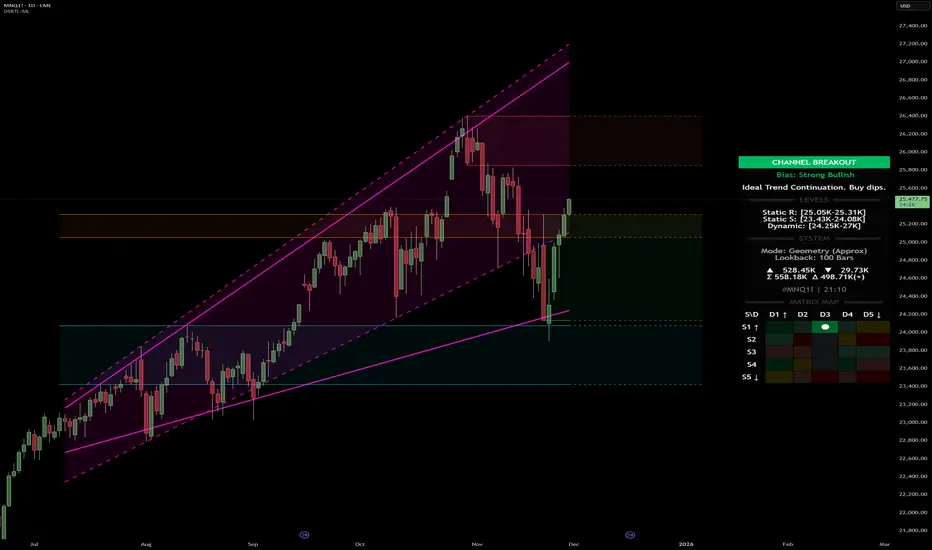
ICT FVG & Order Flow (IRL to ERL)Overview
Master liquidity with precision. This indicator brings the iCT trading concept to life by automatically detecting liquidity pools, fair value gaps, and key swing points. It shows you exactly where price is likely to move next — from Internal Range Liquidity (IRL) to External Range Liquidity (ERL). With built-in alerts and multi-timeframe validation, it helps you stay one step ahead of the market.
Concept
Markets move where liquidity is. According to iCT theory, price usually sweeps internal liquidity (IRL) first and then hunts for external liquidity (ERL). By mapping this process in real time, the indicator provides a clear framework for understanding market structure, liquidity grabs, and directional bias.
How it works
Detects the High-Probability Leg (HPL) — the leg containing a fair value gap (FVG)
Highlights unmitigated FVGs within the current context.
Marks swing points (SPs), IRL levels, and ERL targets automatically.
Identifies IRL rejections when liquidity is taken inside the leg.
Identifies if a FVG is Respected or Disrespected by 2 Candle Rejection (2CR)
Notifies you of every critical liquidity event:
New context leg
New FVG
IRL rejection
ERL or SP liquidity sweep
FVG is Respected or Disrespected by 2CR
Key Features
Automatic drawing of IRL, ERL, and SP levels
FVG types: Simple FVG or Breakaway Gap (BAG)
Multi-timeframe sweep check – if a single candle takes both IRL and ERL, the indicator zooms into a lower timeframe to confirm which liquidity was swept first
Fully customizable alerts for all liquidity events
Flexible settings for swing points, lookback depth, colors, and style
How to use
Start from the monthly chart to define the macro trend.
Analyze the latest order flow leg:
Bullish FVG = bullish context
Bearish FVG = bearish context
Step down to the daily timeframe and repeat the analysis.
Wait for price to approach or reject from IRL (the indicator highlights it automatically).
Drop to a lower timeframe for entries — use timeframe alignment to select the right LTF.
Enter with the FVG model, targeting liquidity within the leg.
Place take profit inside the context — e.g., never above ERL in a bullish setup.
🔔 Alerts
New Context
New FVG
IRL Rejection
ERL Sweep
SP Sweep
2CR
⚙️ Customization
Context side (auto/manual)
LTF pointer (auto/manual)
Show/hide Resistance FVG, Overlapping Defense, ERL/SP sweeps, 2CR
Look back bars, swing lines, swing length, line offsets
* Full color customization (FVG, bullish/bearish, labels, boxes)

Order Flow AnalysisOrder Flow Pressure Suite — Wick, Volume & Absorption-Based Pressure Map
This indicator builds a composite buying/selling pressure score from candle structure, volume behavior, and absorption signals.
It is designed to infer the “intent” behind price moves by looking at how candles form, where they close, and how volume behaves — even without access to true bid/ask or footprint data.
Core Concepts
Wick-to-Body Analysis
The script evaluates the ratio of upper and lower wicks to the total candle range.
Strong wicks with relatively small bodies are treated as rejections :
Long upper wick → potential selling pressure / rejection of higher prices
Long lower wick → potential buying pressure / rejection of lower prices
Close Position Analysis
The close is normalized within the candle range:
Close near the high → bullish pressure
Close near the low → bearish pressure
Close near the middle → more neutral , context taken from wicks and volume
Volume Delta Estimation
Since true bid/ask data is not available on standard charts, the script estimates “volume delta” by distributing total volume between buyers and sellers based on candle characteristics:
Bull candles receive more “buying volume,” weighted toward closes near the high
Bear candles receive more “selling volume,” weighted toward closes near the low
This is an approximation of order flow, not a direct time & sales feed.
Absorption Detection
The script looks for candles where volume is high but price movement is relatively small .
This combination often suggests:
Bullish absorption → buyers absorbing aggressive selling (potential accumulation)
Bearish absorption → sellers absorbing aggressive buying (potential distribution)
Absorption zones are tracked over a configurable lookback and can be shaded in the background.
Composite Pressure Oscillator
All the above components (wicks, close position, heuristic volume delta, absorption bias) are blended into a single pressure score :
Values > 0 → net buying pressure
Values < 0 → net selling pressure
The raw score is smoothed with an EMA to reduce noise and create a cleaner oscillator line.
Divergence Detection
The indicator compares price pivots to pressure pivots:
Bullish divergence : price makes a lower low while pressure makes a higher low
Bearish divergence : price makes a higher high while pressure makes a lower high
These conditions can help highlight potential exhaustion or hidden participation from larger players.
Visual Elements
Histogram showing the intensity of buying/selling pressure
Color-coding for increasing vs. decreasing pressure
Background shading for detected absorption zones
Status table summarizing current pressure, trend bias, volume delta, wick signal, and absorption state in real time
How To Use
Use the pressure oscillator to gauge whether the current bar sequence is dominated by buyers or sellers. Strong positive readings may indicate sustained buying pressure; strong negatives may indicate sustained selling pressure.
Watch for divergences between price and the pressure oscillator around key levels, swings, or zones you already care about.
Use absorption zones and wick rejection signals as additional context around support/resistance, breakouts, or failed moves.
Treat all signals as context and confluence , not as stand-alone trade entries or exits. This tool is best used alongside your existing price action, volume, and risk management framework.
Important Notes & Limitations
This script does not access real bid/ask, footprint, or order book data . All volume delta and absorption interpretations are heuristic estimates derived from OHLCV candles.
Signals are probabilistic , not guarantees. They can be early, late, or outright wrong in fast or low-liquidity markets.
Always validate signals with your own analysis, timeframe alignment, and risk management. This indicator is intended as an analytical tool , not financial advice.

Filter Bar1. Indicator Name
Filter Bar
2. One-line Introduction
A trend-aware bar coloring system that visualizes market direction and strength through adaptive transparency based on regression scoring.
3. General Overview
Filter Bar+ is a minimalist but powerful trend visualization tool that colors chart bars according to market direction and momentum strength.
It analyzes the linear regression trend alignment over a specified lookback period and uses a pairwise comparison algorithm to determine whether the market is in a bullish, bearish, or neutral state.
The result is a "trend score" that gets normalized to reflect trend intensity (0~1).
Bar colors are then dynamically updated using the specified bullish or bearish base colors, where higher intensity results in more opaque (darker) bars, and weaker trends lead to lighter, faded tones.
If no strong trend is detected, bars are shown in gray, signaling indecision or neutrality.
The strength of this indicator lies in its simplicity—it doesn’t draw lines, waves, or shapes, but overlays insight directly onto the chart through smart color cues.
It’s particularly effective as a background filter for price action traders, scalpers, and anyone who prefers clean charts but still wants embedded directional context.
4. Key Advantages
🎨 Adaptive Bar Coloring
Bar color opacity increases with trend strength, offering instant visual confirmation without clutter.
📊 Quantified Trend Direction
Uses a regression-based scoring system to reliably detect uptrends, downtrends, or sideways markets.
⚖️ Customizable Sensitivity
Parameters like lookback period and tolerance percentage give users full control over signal responsiveness.
🧼 Clean Chart Presentation
No lines, shapes, or overlays—just color-coded bars that blend into your existing chart setup.
🚀 Lightweight & Fast
Minimal computational load ensures it works smoothly even on lower-end devices or multiple chart setups.
🔒 Secure Internal Logic
Algorithm is neatly encapsulated and optimized, with no critical logic exposed.
📘 Indicator User Guide
📌 Basic Concept
Filter Bar+ evaluates trend direction and strength using a pairwise comparison of linear regression values.
The result determines whether the market is bullish, bearish, or neutral, and adjusts bar colors accordingly.
It visually amplifies the current market state without drawing any indicators on the chart.
⚙️ Settings Explained
Lookback Period: Number of bars used to compare regression values
Range Tolerance (%): Minimum score required to label a trend as bullish or bearish
Regression Source: Data input used for regression (default: close)
Linear Regression Length: Period for generating the base regression line
Bull/Bear Base Colors: Choose colors to represent bullish or bearish bars
📈 Buy Timing Example
Bars are green (or user-set bullish color) and becoming more vivid
Indicates a strengthening bullish trend; helpful when used alongside breakout confirmation or support zones
📉 Sell Timing Example
Bars turn red (or your custom bearish color) with increasing opacity
Signals growing bearish pressure; acts as confirmation during short setups or breakdowns
🧪 Recommended Use Cases
Combine with volume, RSI, or price action setups for direction filtering
Ideal for clean chart strategies where visual simplicity is preferred
Use as a confirmation layer to reduce noise in sideways markets
🔒 Precautions
This is a visual filter, not a signal generator—use alongside other strategies for entries/exits
In choppy markets, bars may flicker between colors—adjust sensitivity as needed
Works best when you already have a directional thesis and want to validate it visually
Always test settings for your asset/timeframe before applying in live trades
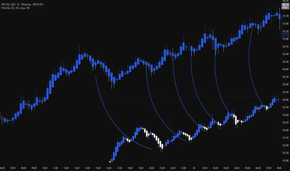
NeuraEdge Block Trades v1.0NEURAEDGE BLOCK TRADES
═══════════════════════════════════════════════════════════════════════
We are excited to release Block Trades!
WHY THIS INDICATOR EXISTS?
Retail traders face a fundamental challenge: institutions move markets, but their activity is hidden. When smart money accumulates at support or distributes at resistance, retail traders often find themselves on the wrong side of the move.
Understanding where institutions are actively buying or selling is crucial for:
• Validating trade setups with volume confirmation
• Identifying supply and demand zones that actually hold
• Avoiding false breakouts driven by retail sentiment
• Spotting accumulation before major moves up
• Detecting distribution before major moves down
Most volume indicators simply show size without context. Block Trades was created to bridge this gap by detecting abnormally large volume bars and determining their directional bias, giving retail traders insight into institutional activity.
═══════════════════════════════════════════════════════════════════════
WHAT IT DOES:
Block Trades identifies volume spikes that likely represent institutional order flow and classifies them as buying pressure, selling pressure, or contested zones. The indicator then validates these prints against directional flow analysis and groups nearby prints into accumulation or distribution clusters.
This helps you answer critical questions:
• Is this support level being defended by institutions?
• Are smart money players distributing into this rally?
• Is heavy volume confirming my trade or warning against it?
• Where are institutional interest zones forming?
KEY FEATURES:
• Multi-tier volume detection (Large: 2x, Huge: 3x, Massive: 5x average)
• Directional classification with flow validation
• Accumulation/distribution zone detection
• Print clustering for institutional interest areas
• Confluence scoring system (0-10 points)
• Real-time statistics dashboard
• Clean, minimal chart labels
═══════════════════════════════════════════════════════════════════════
HOW IT WORKS:
VOLUME SPIKE DETECTION
The indicator monitors volume against a moving average baseline. When current volume significantly exceeds this average (default thresholds: 2x, 3x, 5x), it flags the bar as a potential institutional print.
DIRECTIONAL CLASSIFICATION
Buy Print: Large volume + closes in top 70% of range
Sell Print: Large volume + closes in bottom 70% of range
Neutral Print: Large volume + mid-range close (absorption/contested)
The close position within the bar's range reveals who won the battle. A bar with massive volume that closes near its high indicates aggressive buying. The same volume closing near the low indicates aggressive selling.
FLOW VALIDATION
Each print is validated against underlying institutional flow calculations. This filters out volume spikes that don't align with directional pressure, significantly reducing false signals. Buy prints require bullish flow, sell prints require bearish flow.
ACCUMULATION & DISTRIBUTION ZONES
When multiple prints occur at similar price levels with consistent direction:
• Repeated buy prints + bullish trend = Accumulation (institutions building positions)
• Repeated sell prints + bearish trend = Distribution (institutions unloading positions)
These zones often become powerful support/resistance levels because institutions have established significant positions there.
PRINT CLUSTERING
The indicator groups nearby prints (within configurable ATR distance) into clusters. When 3 or more prints form a cluster, it marks an institutional interest zone. These clusters frequently act as price magnets and reversal points.
PRINT CLUSTERING
The indicator groups nearby prints (within configurable ATR distance) into clusters. When 3 or more prints form a cluster, it marks an institutional interest zone. These clusters frequently act as price magnets and reversal points.
CONFLUENCE SCORING
Each print receives a confluence score (0-10 points) based on:
• Volume size (Massive: +3, Huge: +2, Large: +1)
• Flow alignment (+2 points, configurable)
• Trend alignment (+1)
• New high/low made (+1)
• Extreme close position (+1)
Prints with 5+ points receive a star marker, indicating ultra-high conviction setups.
═══════════════════════════════════════════════════════════════════════
HOW TRADERS USE IT:
USE CASE 1: TRADE VALIDATION
Your system signals a long entry at support. Check Block Trades:
• Buy prints present at this level? Institutions defending = Take the trade
• Sell prints present? Institutions distributing = Skip or wait
• No prints? Proceed with normal risk management
USE CASE 2: IDENTIFYING EXHAUSTION
Price rallies to resistance with heavy volume:
• Sell prints appear = Distribution, institutions unloading into strength
• Likely reversal coming, consider shorts or exit longs
• Confirmed by multiple sell prints = High conviction reversal setup
USE CASE 3: FINDING SUPPORT/RESISTANCE
Accumulation cluster forms at 450 level:
• Multiple buy prints over several sessions
• Institutions building positions at this price
• 450 becomes high-probability support for future pullbacks
• Use for entries or stop placement
USE CASE 4: BREAKOUT CONFIRMATION
Price breaks above key resistance:
• Buy print on breakout bar = Real institutional participation
• High confluence score (5+) = Ultra-high conviction
• Fake breakout would show sell prints or no prints
USE CASE 5: AVOIDING TRAPS
Price spikes up on huge volume:
• Sell print appears (closes low in range) = Trap
• Institutions selling into retail FOMO
• Avoid chasing, prepare for reversal
═══════════════════════════════════════════════════════════════════════
VISUAL ELEMENTS:
ON-CHART LABELS
Buy Print: Green label below bar showing size (LARGE/HUGE/MASSIVE)
Sell Print: Red label above bar showing size
Contested Print: Orange label at bar high (large volume, mid-range close)
Accumulation: Green "ACCUM" label with diamond symbol
Distribution: Red "DISTRIB" label with diamond symbol
WHAT CONTESTED MEANS:
When a bar has massive volume but closes in the middle of its range (neither top nor bottom 70%), it indicates a battle between buyers and sellers with no clear winner. This often occurs at:
• Major support/resistance levels where institutions are absorbing supply/demand
• Transition zones before a directional move
• Areas of genuine price discovery and uncertainty
Contested prints can signal absorption (institutions quietly building positions) or genuine indecision. Watch for follow-through on the next bar to determine which side won.
LABEL MODIFIERS
∆ checkmark = Flow validated (institutional flow aligns with print)
Star symbol = High confluence (5+ points, ultra-high conviction)
CLUSTER ZONES
Semi-transparent boxes marking areas where multiple prints occurred
Extend to the right to show ongoing institutional interest zones
Color-coded: green for bullish clusters, red for bearish clusters
DASHBOARD (TOP RIGHT)
• Current volume state and ratio
• Institutional flow direction
• Cumulative trend direction
• Recent print count (last 20 bars)
• Active cluster count
• Volume thresholds
STATISTICS (BOTTOM LEFT)
• Total session prints
• Buy/sell percentage split
═══════════════════════════════════════════════════════════════════════
SETTINGS:
PRINT DETECTION
• Volume Lookback Period: 20 bars (for average calculation)
• Large Print Threshold: 2.0x average
• Huge Print Threshold: 3.0x average
• Massive Print Threshold: 5.0x average
• Min Candle Size: 0.3x ATR (filters doji bars)
CLASSIFICATION
• Directional Threshold: 70% (how far in range to qualify as buy/sell)
• Show Neutral Prints: Toggle contested zones
• Require New High/Low: Optional stricter filter
INSTITUTIONAL FLOW
• Enable Flow Confluence: On/Off toggle
• Flow Confluence Weight: 2 points (adjustable 1-5)
CLUSTERING
• Enable Clustering: On/Off
• Cluster Distance: 1.0x ATR (how close prints must be)
• Min Prints for Cluster: 3 prints
• Show Cluster Zones: On/Off
DISPLAY
• Show Print Labels: Toggle all labels
• Show Accumulation/Distribution/Contested Labels: Toggle special labels
• Label Size: Tiny/Small/Normal
• Colors: Customizable buy/sell/neutral colors
FILTERS
• Minimum Volume: 0 (set threshold to ignore low volume bars)
• Session Filter: Avoid first/last 15 minutes (low liquidity)
═══════════════════════════════════════════════════════════════════════
BEST PRACTICES:
DO:
✓ Use as confluence with your primary trading system
✓ Pay attention to accumulation/distribution zones
✓ Look for high confluence prints (5+ stars)
✓ Validate breakouts with print direction
✓ Use cluster zones as future support/resistance
✓ Combine with higher timeframe analysis
✓ Works best on liquid instruments (major pairs, indices, large cap stocks)
DON'T:
✗ Trade prints as standalone buy/sell signals
✗ Ignore the directional classification (context matters)
✗ Use on low-volume instruments (prints less reliable)
✗ Chase every print without confluence confirmation
✗ Trade during low liquidity hours (first/last 15 min)
✗ Expect 100% accuracy (it's a confluence tool, not crystal ball)
OPTIMAL TIMEFRAMES:
• 5-minute to 1-hour charts for intraday trading
• 1-hour to 4-hour charts for swing trading
• Daily charts for position trading
BEST INSTRUMENTS:
• Major forex pairs (EUR/USD, GBP/USD, etc.)
• Index futures (ES, NQ, YM)
• High-volume stocks (SPY, QQQ, TSLA, AAPL, etc.)
• Major cryptocurrencies (BTC, ETH)
═══════════════════════════════════════════════════════════════════════
IMPORTANT DISCLAIMERS
METHODOLOGY DISCLAIMER
This indicator identifies abnormally large volume bars and estimates their directional bias based on price action and flow analysis. It does NOT have access to:
• Actual dark pool transaction data
• Off-exchange Alternative Trading System (ATS) prints
• Level 2 order book data
• Individual trade sizes or timestamps
• Institutional order identification
The prints detected are estimates based on publicly available volume and price data from TradingView. They indicate probable institutional activity patterns but are not confirmed block trades or dark pool executions.
USAGE DISCLAIMER
Block Trades is designed as a CONFLUENCE tool to validate trade setups - not as a standalone trading system. The indicator does not:
• Generate specific entry/exit signals
• Provide stop loss or take profit levels
• Constitute a complete trading strategy
• Guarantee profitable trades
Prints should be interpreted within the context of:
• Your overall trading strategy
• Market structure and trend
• Support/resistance levels
• Risk management rules
• Multiple timeframe analysis
RISK DISCLAIMER
Trading involves substantial risk of loss and is not suitable for every investor. Past performance is not indicative of future results. This indicator is a tool for technical analysis only and does NOT constitute financial advice, investment advice, trading advice, or a recommendation to buy or sell any securities or financial instruments.
You should not make any investment decision without conducting your own research and due diligence. The accuracy, completeness, and timeliness of the information provided by this indicator is not guaranteed. No representation is being made that using this indicator will guarantee profits or prevent losses.
By using this indicator, you acknowledge that you understand and accept all risks associated with trading, and you agree that the developer is not liable for any losses you may incur.
═══════════════════════════════════════════════════════════════════════
ALERTS
Available alert conditions:
• Massive Buy Print
• Massive Sell Print
• Huge Buy Print
• Huge Sell Print
• Accumulation Detected
• Distribution Detected
• High Confluence Buy (5+ points)
• High Confluence Sell (5+ points)
Happy Trading!

Multi Timeframe Bollinger Bands Spectrum [Ata]Multi-Timeframe Bollinger Bands Spectrum
Technical Overview
This script integrates multi-timeframe volatility analysis with volume-derived order flow estimation. By combining Bollinger Bands (statistical deviation) with internal candle volume logic, the indicator qualifies price movements to differentiate between sustained trends, reversals, and exhaustion events.
The system is designed to provide a structural context for price action, visualizing market regimes through a dual-zone spectrum and filtering signals based on the interaction between price location and specific volume thresholds.
Core Logic & Calculation
1. Volume Decomposition Algorithm
Instead of using total volume, the script estimates Buying Pressure vs. Selling Pressure based on the close position relative to the candle's High/Low range:
- Buying Volume (vb): Increases as the close approaches the High.
- Selling Volume (vs): Increases as the close approaches the Low.
This logic allows the detection of directional flow even within standard volume bars.
2. Statistical Spectrum
The indicator renders deviations from the Basis (SMA) as two distinct zones:
- Bullish Zone (Blue): Price positioning between the Basis and Upper Band.
- Bearish Zone (Red): Price positioning between the Basis and Lower Band.
This structure is applied across multiple timeframes (overlay) to visualize the macro trend context without noise.
3. Non-Repainting Execution
To ensure historical accuracy and reliability for backtesting, all higher-timeframe data is requested using "lookahead_off". Signals are confirmed only upon the closure of the respective timeframe's candle.
Signal Definitions
Signals are generated only when specific Volatility and Volume conditions intersect:
Reversal Setups (Reaction to Liquidity)
- WALL: Triggered when price rejects the Upper Band accompanied by Extreme Selling Volume (vs > Limit). This suggests active limit sell orders absorbing the rally.
- FLOOR: Triggered when price rejects the Lower Band accompanied by Extreme Buying Volume (vb > Limit). This suggests active limit buy orders absorbing the drop.
- ABSORP: Identifies absorption near the lower bands where selling pressure is met with passive buying (indicated by lower wicks and relative buy volume).
Momentum Setups (Trend Continuation)
- POWER: Validates a breakout above the Upper Band only if supported by Dominant Buying Volume and a strong candle body.
- PANIC: Validates a breakdown below the Lower Band only if supported by Dominant Selling Volume.
- TRAP: Marks failed breakouts where price exits the bands but volume analysis contradicts the move (e.g., low directional volume).
Exhaustion Setups (Statistical Extremes)
- CLIMAX/CRASH: Identifies anomalies where price deviates significantly from the mean (Extreme Deviation) or when volume reaches unsustainable levels relative to the average, often preceding a mean reversion.
Input Parameters
- Bollinger Logic: Configuration for Length and Standard Deviation Multiplier.
- Volume Thresholds: Adjustable factors for Minimum Volume (Trend) and Extreme Volume (Reversal/Climax).
- Timeframe Layers: Toggle visibility for up to 5 higher timeframes.
- Theme: Adjusts label contrast for Dark/Light backgrounds.
Disclaimer
This indicator is strictly for analytical purposes. It provides a visualization of past market data based on statistical and volumetric formulas. Users should apply their own risk management protocols.
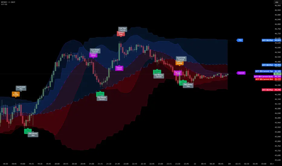
Smart Money Volume Matrix [Ata]Smart Money Volume Matrix
The Smart Money Volume Matrix (SMV Matrix) is an advanced volume-spread analysis (VSA) dashboard and charting tool designed to identify significant market anomalies by analyzing the relationship between price extremes and volume flow.
Unlike traditional indicators that rely solely on moving averages or oscillators, this tool performs a "Snapshot Analysis" of a defined lookback period (default: 100 bars) to rank price action based on Order Flow Dominance. It isolates the Top 10 Highest and Lowest Close prices and scrutinizes the volume behind them to categorize market sentiment into four distinct phases: Distribution, No Demand, Absorption, and Exhaustion.
Core Logic & Methodology
The script operates on a Zero-Lag Snapshot Engine. It does not print historical signals bar-by-bar; instead, it evaluates the current market structure relative to the recent history (Lookback Period).
1. Ranking Engine: The script scans the lookback period to find the Top 10 Highest Closes and Top 10 Lowest Closes.
2. Volume Classification: For each ranked bar, it calculates the "Intrabar Buy/Sell Volume" (or approximates it using candle geometry if Intrabar data is unavailable).
3. Dominance Detection: It compares Buying Volume vs. Selling Volume to determine who is in control at critical price levels.
Signal Classifications (VSA Logic)
The indicator generates labels on the chart and updates the dashboard table based on the following logic:
1. At Price Tops (Resistance Areas):
- Distribution (Supply): High Price + High Total Volume + Sellers Dominant.
Interpretation: Indicates heavy institutional selling into rising prices. Often precedes a reversal.
- Buy Climax: High Price + High Total Volume + Buyers Dominant.
Interpretation: Extreme buying frenzy. While bullish, it often marks a "trap" or temporary top due to exhaustion.
- No Demand: High Price + Low Volume.
Interpretation: Prices drifted higher but lack institutional participation. A sign of weakness.
2. At Price Bottoms (Support Areas):
- Absorption: Low Price + High Total Volume + Buyers Dominant.
Interpretation: Institutional money is absorbing selling pressure (passive buying). A strong sign of accumulation.
- Panic Sell: Low Price + High Total Volume + Sellers Dominant.
Interpretation: Extreme fear. High volume at lows typically indicates capitulation and potential hands-changing.
- Exhaustion: Low Price + Low Volume.
Interpretation: Selling pressure has dried up. The market may float upward due to lack of sellers.
Key Features
- Dashboard Matrix Table:
Displays the exact Close Price, Buy/Sell Volume, and Market State (Group) for the Top 10 ranking bars.
Smart Footer: Automatically detects the active "Resistance Zone" (derived from G1 Distribution levels) and "Support Zone" (derived from G3 Absorption levels) and reports the current price status relative to these zones (e.g., "Testing Resistance", "Breakout", "At Support").
- Smart Zones (Auto S/R):
Automatically draws Support and Resistance boxes extending into the future based on the most significant volume clusters found in the rankings. Includes logic to detect "Flips" (e.g., when Support breaks, it is labeled as a flip to Resistance).
- Average Trend Channels:
Calculates a Linear Regression trend line based specifically on the coordinates of the Top 10 Highs and Top 10 Lows, providing a "Best Fit" channel for the current market structure.
- Visual Clarity:
Labels utilize a "Smart Stacking" algorithm to prevent overlap on the chart. Guide lines connect labels to their respective candles for precise identification.
Settings & Configuration
- Matrix Settings: Lookback Period (default 100 bars) and Top Rank Count.
- Volume Engine: Choose between "Intrabar (Precise)" for accurate order flow or "Geometry (Approx)" for standard volume estimation.
- Visuals: Toggle Table, Labels, Lines, Zones, and Trend Lines. Adjust transparency and font sizes.
IMPORTANT NOTE ON SNAPSHOT LOGIC
This indicator is designed as a Real-Time Dashboard. It continuously updates the "Top 10" list as new candles form. Therefore, a label that appears on a candle may disappear if that candle falls out of the Top 10 ranking or leaves the lookback window. This is intended behavior to ensure the chart always reflects the current most critical levels, rather than a historical record of past signals. It is best used for live market analysis rather than historical back testing.
Disclaimer: This tool is for educational and analytical purposes only. Volume analysis is subjective and should be used in conjunction with other methods of technical analysis.
