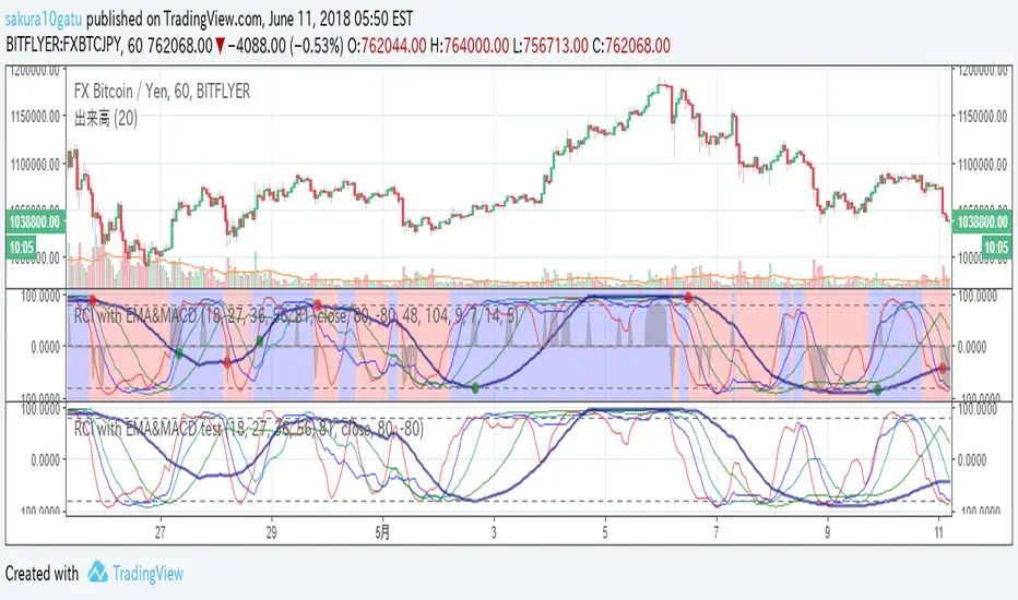
RCI with EMA&MACD2018/6/11 Re-release for house rule of Trading view.
5lines : RCI lines. A thick navy line has the longest period.
circles : MACD cross. GC=green DC=red
backcolor : Short EMA > Long EMA is blue. Short EMA < Long EMA is red.
Black shadow : It reveals its appearance when over-buying/selling.
It helps your entry.
在腳本中搜尋"2018年4月至8月伦敦金现跌幅+期间贵金属指数表现"
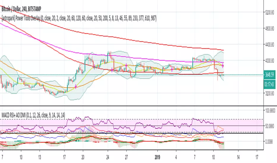
[astropark] Power Tools Overlay//******************************************************************************
// Power Tools Overlay
// Inner Version 1.2.1 13/12/2018
// Developer: iDelphi
// Developer: astropark (Ichimoku Cloud), SMA EMA & Cross tools
//------------------------------------------------------------------------------
// 21/11/2018 Added EMA SMA WMA
// 21/11/2018 Added SMA-EMA EMA-WMA WMA-SMA (Thanks to mariobros1 for the idea of the Simultaneous MA)
// 21/11/2018 Added Bollinger Bands
// 21/11/2018 Added Ichimoku Cloud (Thanks to astropark for all the code of the Ichimoku Cloud)
// 23/11/2018 Show all the indicator as default
// 23/11/2018 Added a cross when single Moving Averages crossing (Thanks to astropark for the idea)
// 24/11/2018 Descriptions Fix
// 24/11/2018 Added Option to enable/disable all Moving Averages
// 10/12/2018 Added EMAs and Crosses
// 13/12/2018 indicator number fixes
//******************************************************************************

[astropark] Power Tools Overlay//******************************************************************************
// Power Tools Overlay
// Inner Version 1.2 20/12/2018
// Developer: iDelphi
// Developer: astropark (Ichimoku Cloud), SMA EMA & Cross tools
//------------------------------------------------------------------------------
// 21/11/2018 Added EMA SMA WMA
// 21/11/2018 Added SMA-EMA EMA-WMA WMA-SMA (Thanks to mariobros1 for the idea of the Simultaneous MA)
// 21/11/2018 Added Bollinger Bands
// 21/11/2018 Added Ichimoku Cloud (Thanks to astropark for all the code of the Ichimoku Cloud)
// 23/11/2018 Show all the indicator as default
// 23/11/2018 Added a cross when single Moving Averages crossing (Thanks to astropark for the idea)
// 24/11/2018 Descriptions Fix
// 24/11/2018 Added Option to enable/disable all Moving Averages
// 10/12/2018 Added EMAs and Crosses
//******************************************************************************

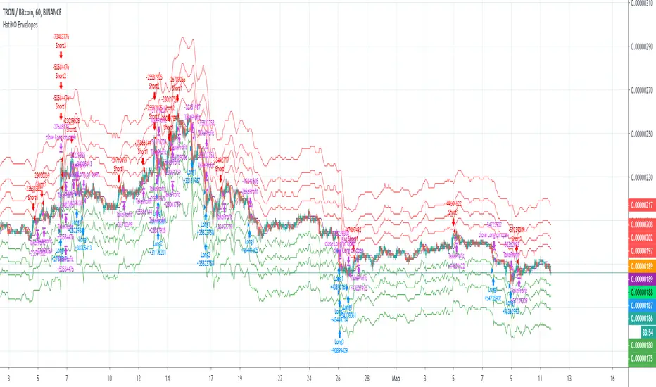
HatiKO EnvelopesPublished source code is subject to the terms of the GNU Affero General Public License v3.0
This script describes and provides backtesting functionality to internal strategy of algorithmic crypto trading software "HatiKO bot".
Suitable for backtesting any Cryptocurrency Pair on any Exchange/Platform, any Timeframe.
Core Mechanics of this strategy are based on theory of price always returning to Moving Average + Envelopes indicator (Moving_average_envelope from Wiki)
Developement of this script and trading software is inspired by:
"Essential Technical Analysis: Tools and Techniques to Spot Market Trends" by Leigh Stevens (published on 12th of April 2002)
"Moving Average Envelopes" by ChartSchool, StockCharts platform (published on 13th of April 2015 or earlier)
"Коля Колеснік" from Crypto Times channel ("Метод сетка", published on 19th of August 2018)
"3 ways to use Moving Average Envelopes" by Rich Fitton, published on Trader's Nest (published on 28st of November 2018 or earlier)
noro's "Robot WhiteBox ShiftMA" strategy v1 script, published on TradingView platform (published on 29th of August 2018)
"Moving Average Envelopes: A Popular Trading Tool" Investopedia article (published 25th of June 2019)
and KROOL1980's blogpost on Argolabs ("Гридерство или Сетка как источник прибыли на форекс", published on 27th of February 2015)
Core Features:
1) Up to 4 Envelopes in each direction (Long/Short)
2) Use any of 6 different basis MAs, optionally use different MAs for Opening and Closure
3) Use different Timeframes for MA calculation, without any repainting and lookahead bias.
4) Fixed order size, not Martingale strategy
5) Close open position earlier by using Deviation parameter
6) PineScript v4 code
Options description:
Lot - % from your initial balance to use for order size calculation
Timeframe Short - Timeframe to use for Short Opening MA calculation, can be chosen from dropdown list, default is Current Graph Timeframe
MA Type Short - Type of MA to use for Short Opening MA calculation, can be chosen from dropdown list, default is SMA
Data Short - Source of Price for Short Opening MA calculation, can be chosen from dropdown list, default is OHLC4
MA Length Short - Period used for Short Opening MA calculation, should be >=1, default is 3
MA offset Short - Offset for MA value used for Short Envelopes calculation, should be >= 0, default is 0
Timeframe Long - Timeframe to use for Long Opening MA calculation, can be chosen from dropdown list, default is Current Graph Timeframe
MA Type Long - Type of MA to use for Long Opening MA calculation, can be chosen from dropdown list, default is SMA
Data Long - Source of Price for Long Opening MA calculation, can be chosen from dropdown list, default is OHLC4
MA Length Long - Period used for Long Opening MA calculation, should be >=1, default is 3
MA offset Long - Offset for MA value used for Long Envelopes calculation, should be >= 0, default is 0
Mode close MA Short - Enable different MA for Short position Closure, default is "false". If false, Closure MA = Opening MA
Timeframe Short Close - Timeframe to use for Short Position Closure MA calculation, can be chosen from dropdown list, default is Current Graph Timeframe
MA Type Close Short - Type of MA to use for Short Position Closure MA calculation, can be chosen from dropdown list, default is SMA
Data Short Close - Source of Price for Short Closure MA calculation, can be chosen from dropdown list, default is OHLC4
MA Length Short Close - Period used for Short Opening MA calculation, should be >=1, default is 3
Short Deviation - % to move from MA value, used to close position above or beyond MA, can be negative, default is 0
MA offset Short Close - Offset for MA value used for Short Position Closure calculation, should be >= 0, default is 0
Mode close MA Long - Enable different MA for Long position Closure, default is "false". If false, Closure MA = Opening MA
Timeframe Long Close - Timeframe to use for Long Position Closure MA calculation, can be chosen from dropdown list, default is Current Graph Timeframe
MA Type Close Long - Type of MA to use for Long Position Closure MA calculation, can be chosen from dropdown list, default is SMA
Data Long Close - Source of Price for Long Closure MA calculation, can be chosen from dropdown list, default is OHLC4
MA Length Long Close - Period used for Long Opening MA calculation, should be >=1, default is 3
Long Deviation - % to move from MA value, used to close position above or beyond MA, can be negative, default is 0
MA offset Long Close - Offset for MA value used for Long Position Closure calculation, should be >= 0, default is 0
Short Shift 1..4 - % from MA value to put Envelopes at, for Shorts numbers should be positive, the higher is number, the higher should be Shift position, example: "Shift 1 = 1, shift 2 = 2, etc."
Long Shift 1..4 - % from MA value to put Envelopes at, for Longs numbers should be negative, the lower is number, the lower should be Shift position, example: "Shift 1 = -1, shift 2 = -2, etc."
From Year 20XX - Backtesting Starting Year number, only 20xx supported as script is cryptocurrency-oriented.
To Year 20XX - Backtesting Final Year number, only 20xx supported as script is cryptocurrency-oriented.
From Month - Years starting Month, optional tweaking, changing not recommended
To Month - Years ending Month, optional tweaking, changing not recommended
From day - Months starting day, optional tweaking, changing not recommended
To day - Months ending day, optional tweaking, changing not recommended
Graph notes:
Green lines - Long Envelopes.
Red lines - Short Envelopes.
Orange line - MA for closing of Short positions.
Lime line - MA for closing of Long positions.
**************************************************************************************************************************************************************************************************************
Опубликованный исходный код регулируется Условиями Стандартной Общественной Лицензии GNU Affero v3.0
Этот скрипт описывает и предоставляет функции бектеста для внутренней стратегии алгоритмического программного обеспечения "HatiKO bot".
Подходит для тестирования любой криптовалютной пары на любой бирже/платформе, на любом таймфрейме.
Кор-механика этой стратегии основана на теории всегда возвращающейся к значению МА цены с использованием индикатора Envelopes (Moving_average_envelope from Wiki)
Разработка этого скрипта и программного обеспечения для торговли вдохновлена следующими источниками:
Книга "Essential Technical Analysis: Tools and Techniques to Spot Market Trends" Ли Стивенса (опубликовано 12 апреля 2002 года)
«Moving Average Envelopes» от ChartSchool, платформа StockCharts (опубликовано 13 апреля 2015 года или раньше)
«Коля Колеснік» с канала Crypto Times («Метод сетка», опубликовано 19 августа 2018 года)
«3 ways to use Moving Average Envelopes» Рича Фиттона, опубликованные в «Trader's Nest» (опубликовано 28 ноября 2018 года или раньше)
Скрипт стратегии noro "Robot WhiteBox ShiftMA" v1, опубликованный на платформе TradingView(опубликовано 29 августа 2018 года)
«Moving Average Envelopes: A Popular Trading Tool», статья Investopedia (опубликовано 25 июня 2019 года)
Блог KROOL1980 из Argolabs («Гридерство или Сетка как источник прибыли на форекс», опубликовано 27 февраля 2015 года)
Основные особенности:
1) До 4-х Ордеров в каждом из направлении (Лонг / Шорт)
2) Выбор из 6-ти разных базовых МА, опционально используйте разные МА для открытия и закрытия.
3) Используйте разные таймфреймы для расчета MA, без перерисовки и "эффекта стеклянного шара".
4) Фиксированный размер ордера, а не стратегия Мартингейла
5) Возможность закрытия открытой позиции заблаговременно, используя параметр Deviation
6) Код реализован на PineScript v4
Описание параметров:
Lot - % от вашего первоначального баланса, используется при расчете размера Ордера
Timeframe Short - таймфрейм, используемый для расчета МА Открытия Шорт позиций, может быть выбран из списка, по умолчанию - таймфрейм текущего графика
MA Type Short - тип MA, используемый для расчета МА Открытия Шорт позиций, может быть выбран из списка, по умолчанию SMA
Data Short - источник цены для расчета МА Открытия Шорт позиций, может быть выбран из списка, по умолчанию OHLC4
MA Length Short - период, используемый для расчета МА Открытия Шорт позиций, должен быть >= 1, по умолчанию 3
MA Offset Short - смещение значения MA, используемого для расчета Шорт Ордеров, должно быть >= 0, по умолчанию 0
Timeframe Long - таймфрейм, используемый для расчета МА Открытия Лонг позиций, может быть выбран из списка, по умолчанию - таймфрейм текущего графика
MA Type Long - тип MA, используемый для расчета МА Открытия Лонг позиций, может быть выбран из списка, по умолчанию SMA
Data Long - источник цены для расчета МА Открытия Лонг позиций, может быть выбран из списка, по умолчанию OHLC4
MA Length Long - период, используемый для расчета МА Открытия Лонг позиций, должен быть >= 1, по умолчанию 3
MA Offset Long - смещение значения MA, используемого для расчета Лонг Ордеров, должно быть >= 0, по умолчанию 0
Mode close MA Short - Включает отдельное MA для закрытия Шорт позиции, по умолчанию «false». Если false, MA Закрытия = MA Открытия
Timeframe Short Close - таймфрейм, используемый для расчета МА Закрытия Шорт позиций, может быть выбран из списка, по умолчанию - таймфрейм текущего графика
MA Type Close Short - тип MA, используемый при расчете МА Закрытия Шорт позиции. Mожно выбрать из списка, по умолчанию SMA
Data Short Close - источник цены для расчета МА Закрытия Шорт позиций, может быть выбран из списка, по умолчанию OHLC4
MA Length Short Close - период, используемый для расчета МА Закрытия Шорт позиции, должен быть >= 1, по умолчанию 3
Short Deviation - % отклонения от значения MA, используется для закрытия позиции выше или ниже рассчитанного значения MA, может быть отрицательным, по умолчанию 0
MA Offset Short Close - смещение значения MA, используемого для расчета закрытия Шорт позиции, должно быть >= 0, по умолчанию 0
Mode close MA Long - Включает разные MA для закрытия Лонг позиции, по умолчанию «false». Если false, MA Закрытия = MA Открытия
Timeframe Long Close - таймфрейм, используемый для расчета МА Закрытия Лонг позиций, может быть выбран из списка, по умолчанию - таймфрейм текущего графика
MA Type Close Long - тип MA, используемый при расчете МА Закрытия Лонг позиции. Mожно выбрать из списка, по умолчанию SMA
Data Long Close - источник цены для расчета МА Закрытия Лонг позиций, может быть выбран из списка, по умолчанию OHLC4
MA Length Long Close - период, используемый для расчета МА Закрытия Лонг позиции, должен быть >= 1, по умолчанию 3
Long Deviation -% для перехода от значения MA, используется для закрытия позиции выше или ниже рассчитанного значения MA, может быть отрицательным, по умолчанию 0
MA Offset Long Close - смещение значения MA, используемого для расчета закрытия Лонг позиции, должно быть >= 0, по умолчанию 0
Short Shift 1..4 - % от значения MA для размещения Ордеров, для Шорт Ордеров должен быть положительным, чем выше номер, тем выше должна располагаться позиция Shift, например: «Shift 1 = 1, Shift 2 = 2 и т.д. "
Long Shift 1..4 - % от значения MA для размещения Ордеров, для Лонг Ордеров должно быть отрицательным, чем ниже число, тем ниже должна располагаться позиция Shift, например: «Shift 1 = -1, Shift 2 = -2, и т.д."
From Year 20XX - Год начала тестирования, из-за ориентированности на криптовалюты поддерживаются только значения формата 20хх.
To Year 20XX - Год окончания тестирования, из-за ориентированности на криптовалюты поддерживаются только значения формата 20хх.
From Month - Начальный месяц, опционально, менять не рекомендуется
To Month - Конечный месяц, опционально, менять не рекомендуется
From day - Начальный день месяца, опционально, менять не рекомендуется
To day - Конечный день месяца, опционально, менять не рекомендуется
Пояснения к графику:
Зеленые линии - Лонг Ордера.
Красные линии - Шорт Ордера.
Оранжевая линия - MA Закрытия Шорт позиций.
Лаймовая линия - MA Закрытия Лонг позиций.
[Delphi] RSI - Dynamic Movement Sys - Volume Oscil - Pista CicCopyright by Delphi v1.0 05/07/2018 - 12/07/2018
RSI - Dynamic Movement System - Volume Oscillator - Pista Ciclica
Follow me for updates and strategies
05/07/2018 Added Pista Ciclica
05/07/2018 Added RSI
09/07/2018 Added ADX - Dynamic Movement System
12/07/2018 Added Volume Oscillator

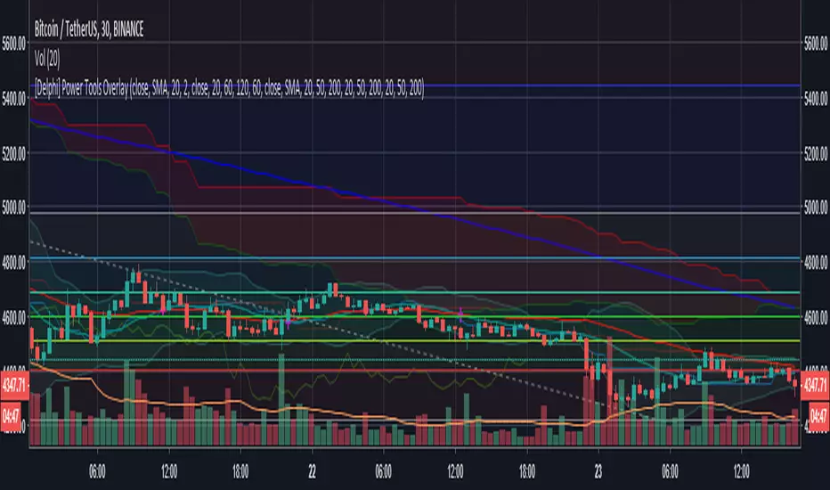
[Delphi] Power Tools OverlayFEATURE
3EMA 3MA 3WMA 3MA-3EMA 3EMA-3WMA 3WMA-3MA
Bollinger Bands
Ichimoku Cloud
//******************************************************************************
// Power Tools Overlay
// Inner Version 1.0 21/11/2018
// Developer: iDelphi
// Developer: astropark (Ichimoku Cloud)
//------------------------------------------------------------------------------
// 21/11/2018 Added EMA MA WMA
// 21/11/2018 Added MA-EMA EMA-WMA WMA-MA (Thanks to mariobros1 for the idea of the Simultaneous MA)
// 21/11/2018 Added Bollinger Bands
// 21/11/2018 Added Ichimoku Cloud (Thanks to astropark for all the code of the Ichimoku Cloud)
//******************************************************************************
Bitcoin Cycle History Visualization [SwissAlgo]BTC 4-Year Cycle Tops & Bottoms
Historical visualization of Bitcoin's market cycles from 2010 to present, with projections based on weighted averages of past performance.
-----------------------------------------------------------------
CALCULATION METHODOLOGY
Why Bottom-to-Bottom Cycle Measurement?
This indicator defines cycles as bottom-to-bottom periods. This is one of several valid approaches to Bitcoin cycle analysis:
- Focuses on market behavior (price bottoms) rather than supply schedule events (halving-to-halving)
- Bottoms may offer good reference points for some analytical purposes
- Tops tend to be extended periods that are harder to define precisely
- Aligns with how some traditional asset cycles are measured and the timing observed in the broader "risk-on" assets category
- Halving events are shown separately (yellow backgrounds) for reference
- Neither halving-based nor bottom-based measurement is inherently superior
Different analysts prefer different cycle definitions based on their analytical goals. This approach prioritizes observable market turning points.
Cycle Date Definitions
- Approximate monthly ranges used for each event (e.g., Nov 2022 bottom = Nov 1-30, 2022)
- Cycle 1: Jul 2010 bottom → Jun 2011 top → Nov 2011 bottom
- Cycle 2: Nov 2011 bottom → Dec 2013 top → Jan 2015 bottom
- Cycle 3: Jan 2015 bottom → Dec 2017 top → Dec 2018 bottom
- Cycle 4: Dec 2018 bottom → Nov 2021 top → Nov 2022 bottom
- Future cycles will be added as new top/bottom dates become firm
Duration Calculations
- Days = timestamp difference converted to days (milliseconds ÷ 86,400,000)
- Bottom → Top: days from cycle bottom to peak
- Top → Bottom: days from peak to next cycle bottom
- Bottom → Bottom: full cycle duration (sum of above)
Price Change Calculations
- % Change = ((New Price - Old Price) / Old Price) × 100
- Example: $200 → $19,700 = ((19,700 - 200) / 200) × 100 = 9,750% gain
- Approximate historical prices used (rounded to significant figures)
Weighted Average Formula
Recent cycles weighted more heavily to reflect the evolved market structure:
- Cycle 1 (2010-2011): EXCLUDED (too early-stage, tiny market cap)
- Cycle 2 (2011-2015): Weight = 1x
- Cycle 3 (2015-2018): Weight = 3x
- Cycle 4 (2018-2022): Weight = 5x
Formula: Weighted Avg = (C2×1 + C3×3 + C4×5) / (1+3+5)
Example for Bottom→Top days: (761×1 + 1065×3 + 1066×5) / 9 = 1,032 days
Projection Method
- Projected Top Date = Nov 2022 bottom + weighted avg Bottom→Top days
- Projected Bottom Date = Nov 2022 bottom + weighted avg Bottom→Bottom days
- Current days elapsed compared to weighted averages
- Warning symbol (⚠) shown when the current cycle exceeds the historical average
Technical Implementation
- Historical cycle dates are hardcoded (not algorithmically detected)
- Dates represent approximate monthly ranges for each event
- The indicator will be updated as the Cycle 5 top and bottom dates become confirmed
- Updates require manual code maintenance - not automatic
- Users should verify they're using the latest version for current cycle data
-----------------------------------------------------------------
FEATURES
- Background highlights for historical tops (red), bottoms (green), and halving events (yellow)
- Data table showing cycle durations and price changes
- Visual cycle boundary boxes with subtle coloring
- Projected timeframes displayed as dashed vertical lines
- Toggle on/off for each visual element
- Customizable background colors
-----------------------------------------------------------------
DISPLAY SETTINGS
- Show/hide cycle tops, bottoms, halvings, data table, and cycle boxes
- Customizable background colors for each event type
- Clean, institutional-grade visual design suitable for analysis
UPDATES & MAINTENANCE
This indicator is maintained as new cycle events occur. When Cycle 5's top and bottom are confirmed with sufficient time elapsed, the code and projections will be updated accordingly. Check for the latest version periodically.
OPEN SOURCE
Code available for review, modification, and improvement. Educational transparency is prioritized.
-----------------------------------------------------------------
IMPORTANT LIMITATIONS
⚠ EXTREMELY SMALL SAMPLE SIZE
Based on only 4 complete cycles (2011-2022). In statistical analysis, this is insufficient for reliable predictions.
⚠ CHANGED MARKET STRUCTURE
Bitcoin's market has fundamentally evolved since early cycles:
- 2010-2015: Tiny market cap, retail-only, unregulated
- 2024-2025: Institutional adoption, spot ETFs, regulatory frameworks, macro correlation
The environment that created past patterns no longer exists in the same form.
⚠ NO PREDICTIVE GUARANTEE
Historical patterns can and do break. Market cycles are not laws of physics. Past performance does not guarantee future results. The next cycle may not follow historical averages.
⚠ LENGTHENING CYCLE THEORY
Some analysts believe cycles are extending over time (diminishing returns, maturing market). If true, simple averaging underestimates future cycle lengths.
⚠ SELF-FULFILLING PROPHECY RISK
The halving narrative may be partially circular - it works because people believe it works. Sufficient changes in market structure or participant behavior can invalidate the pattern.
⚠ APPROXIMATE DATA
Historical prices rounded to significant figures. Exact bottom/top dates vary by exchange. Month-long ranges are used for simplicity.
EDUCATIONAL USE ONLY
This indicator is designed for historical analysis and understanding Bitcoin's past behavior. It is NOT:
- Trading advice or financial recommendations
- A guarantee or prediction of future price movements
- Suitable as a sole basis for investment decisions
- A replacement for fundamental or technical analysis
The projections show "what if the pattern continues exactly" - not "what will happen."
Always conduct independent research, understand the risks, and consult qualified financial advisors before making investment decisions. Only invest what you can afford to lose.

Traders Reality Rate Spike Monitor 0.1 betaTraders Reality Rate Spike Monitor
## **Early Warning System for Interest Rate-Driven Market Crashes**
Based on critical market analysis revealing the dangerous correlation between interest rate spikes and major market selloffs, this indicator provides **three-tier alerts** for US 10-Year Treasury yield acceleration.
### **📊 Key Market Intelligence:**
**Historical Precedent:** The 2018 market crash occurred when unrealized bank losses hit $256 billion with interest rates at just 2.5%. **Current unrealized losses have reached $560 billion** - more than double the 2018 levels - while rates sit at 4.5%.
**Critical Vulnerabilities:**
- **$559 billion in tech sector debt** maturing through 2025
- **65% of investment-grade debt** rated BBB (vulnerable to adverse conditions)
- **$9.5 trillion in total debt** requiring refinancing
- Every 1% rate increase costs the economy **$360 billion annually**
### **🚨 Alert System:**
**📊 WATCH (20+ basis points/3 days):** Early positioning signal
**⚠️ WARNING (30+ basis points/3 days):** Prepare for volatility
**🚨 CRITICAL (40+ basis points/3 days):** Historical crash threshold
### **💡 Why This Matters:**
Interest rate spikes historically trigger major market corrections:
- **2018:** 70 basis points spike → 20% S&P 500 crash
- **2025:** Similar pattern led to massive selloffs
- **Current risk:** 2x higher unrealized losses than 2018
### **⚡ Features:**
✅ **Zero chart clutter** - invisible until alerts trigger
✅ **Dynamic calculation** - automatically adjusts to current yield levels
✅ **Multi-timeframe compatibility** - works on any chart timeframe
✅ **Professional alerts** - with actual basis point calculations
### **🎯 Use Case:**
Perfect for traders and investors who understand that **debt refinancing pressure** and **unrealized bank losses** create systemic risks that manifest through interest rate volatility. When rates spike rapidly, leveraged positions unwind and markets crash.
**"Every point costs us $360 billion a year. Think of that."** - This indicator helps you see those critical rate movements before the market does.
---
**Disclaimer:** This indicator is for educational purposes. Past performance does not guarantee future results. Always manage risk appropriately.
---
This description positions your indicator as a **serious professional tool** based on real market analysis rather than just another technical indicator! 🚀

JPMorgan G7 Volatility IndexThe JPMorgan G7 Volatility Index: Scientific Analysis and Professional Applications
Introduction
The JPMorgan G7 Volatility Index (G7VOL) represents a sophisticated metric for monitoring currency market volatility across major developed economies. This indicator functions as an approximation of JPMorgan's proprietary volatility indices, providing traders and investors with a normalized measurement of cross-currency volatility conditions (Clark, 2019).
Theoretical Foundation
Currency volatility is fundamentally defined as "the statistical measure of the dispersion of returns for a given security or market index" (Hull, 2018, p.127). In the context of G7 currencies, this volatility measurement becomes particularly significant due to the economic importance of these nations, which collectively represent more than 50% of global nominal GDP (IMF, 2022).
According to Menkhoff et al. (2012, p.685), "currency volatility serves as a global risk factor that affects expected returns across different asset classes." This finding underscores the importance of monitoring G7 currency volatility as a proxy for global financial conditions.
Methodology
The G7VOL indicator employs a multi-step calculation process:
Individual volatility calculation for seven major currency pairs using standard deviation normalized by price (Lo, 2002)
- Weighted-average combination of these volatilities to form a composite index
- Normalization against historical bands to create a standardized scale
- Visual representation through dynamic coloring that reflects current market conditions
The mathematical foundation follows the volatility calculation methodology proposed by Bollerslev et al. (2018):
Volatility = σ(returns) / price × 100
Where σ represents standard deviation calculated over a specified timeframe, typically 20 periods as recommended by the Bank for International Settlements (BIS, 2020).
Professional Applications
Professional traders and institutional investors employ the G7VOL indicator in several key ways:
1. Risk Management Signaling
According to research by Adrian and Brunnermeier (2016), elevated currency volatility often precedes broader market stress. When the G7VOL breaches its high volatility threshold (typically 1.5 times the 100-period average), portfolio managers frequently reduce risk exposure across asset classes. As noted by Borio (2019, p.17), "currency volatility spikes have historically preceded equity market corrections by 2-7 trading days."
2. Counter-Cyclical Investment Strategy
Low G7 volatility periods (readings below the lower band) tend to coincide with what Shin (2017) describes as "risk-on" environments. Professional investors often use these signals to increase allocations to higher-beta assets and emerging markets. Campbell et al. (2021) found that G7 volatility in the lowest quintile historically preceded emerging market outperformance by an average of 3.7% over subsequent quarters.
3. Regime Identification
The normalized volatility framework enables identification of distinct market regimes:
- Readings above 1.0: Crisis/high volatility regime
- Readings between -0.5 and 0.5: Normal volatility regime
- Readings below -1.0: Unusually calm markets
According to Rey (2015), these regimes have significant implications for global monetary policy transmission mechanisms and cross-border capital flows.
Interpretation and Trading Applications
G7 currency volatility serves as a barometer for global financial conditions due to these currencies' centrality in international trade and reserve status. As noted by Gagnon and Ihrig (2021, p.423), "G7 currency volatility captures both trade-related uncertainty and broader financial market risk appetites."
Professional traders apply this indicator in multiple contexts:
- Leading indicator: Research from the Federal Reserve Board (Powell, 2020) suggests G7 volatility often leads VIX movements by 1-3 days, providing advance warning of broader market volatility.
- Correlation shifts: During periods of elevated G7 volatility, cross-asset correlations typically increase what Brunnermeier and Pedersen (2009) term "correlation breakdown during stress periods." This phenomenon informs portfolio diversification strategies.
- Carry trade timing: Currency carry strategies perform best during low volatility regimes as documented by Lustig et al. (2011). The G7VOL indicator provides objective thresholds for initiating or exiting such positions.
References
Adrian, T. and Brunnermeier, M.K. (2016) 'CoVaR', American Economic Review, 106(7), pp.1705-1741.
Bank for International Settlements (2020) Monitoring Volatility in Foreign Exchange Markets. BIS Quarterly Review, December 2020.
Bollerslev, T., Patton, A.J. and Quaedvlieg, R. (2018) 'Modeling and forecasting (un)reliable realized volatilities', Journal of Econometrics, 204(1), pp.112-130.
Borio, C. (2019) 'Monetary policy in the grip of a pincer movement', BIS Working Papers, No. 706.
Brunnermeier, M.K. and Pedersen, L.H. (2009) 'Market liquidity and funding liquidity', Review of Financial Studies, 22(6), pp.2201-2238.
Campbell, J.Y., Sunderam, A. and Viceira, L.M. (2021) 'Inflation Bets or Deflation Hedges? The Changing Risks of Nominal Bonds', Critical Finance Review, 10(2), pp.303-336.
Clark, J. (2019) 'Currency Volatility and Macro Fundamentals', JPMorgan Global FX Research Quarterly, Fall 2019.
Gagnon, J.E. and Ihrig, J. (2021) 'What drives foreign exchange markets?', International Finance, 24(3), pp.414-428.
Hull, J.C. (2018) Options, Futures, and Other Derivatives. 10th edn. London: Pearson.
International Monetary Fund (2022) World Economic Outlook Database. Washington, DC: IMF.
Lo, A.W. (2002) 'The statistics of Sharpe ratios', Financial Analysts Journal, 58(4), pp.36-52.
Lustig, H., Roussanov, N. and Verdelhan, A. (2011) 'Common risk factors in currency markets', Review of Financial Studies, 24(11), pp.3731-3777.
Menkhoff, L., Sarno, L., Schmeling, M. and Schrimpf, A. (2012) 'Carry trades and global foreign exchange volatility', Journal of Finance, 67(2), pp.681-718.
Powell, J. (2020) Monetary Policy and Price Stability. Speech at Jackson Hole Economic Symposium, August 27, 2020.
Rey, H. (2015) 'Dilemma not trilemma: The global financial cycle and monetary policy independence', NBER Working Paper No. 21162.
Shin, H.S. (2017) 'The bank/capital markets nexus goes global', Bank for International Settlements Speech, January 15, 2017.

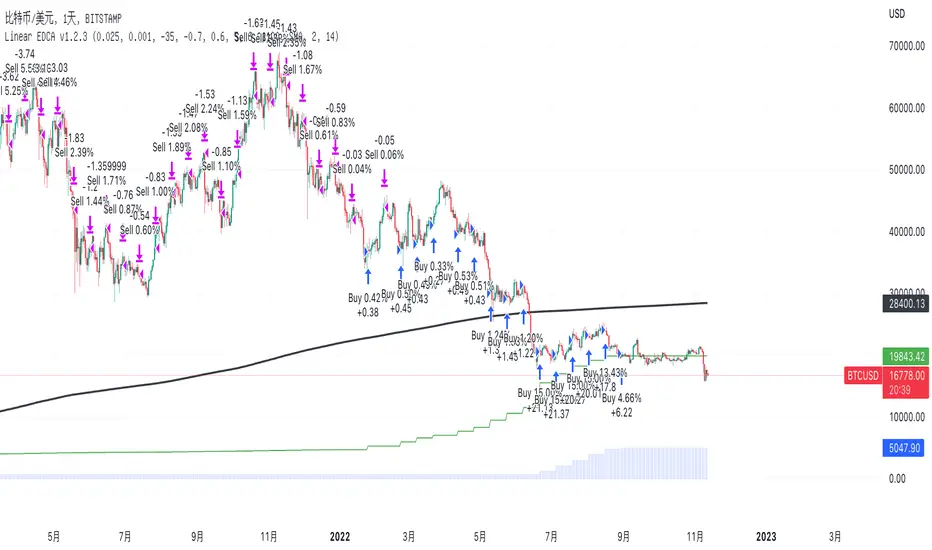
Linear EDCA v1.2Strategy Description:
Linear EDCA (Linear Enhanced Dollar Cost Averaging) is an enhanced version of the DCA fixed investment strategy. It has the following features:
1. Take the 1100-day SMA as a reference indicator, enter the buy range below the moving average, and enter the sell range above the moving average
2. The order to buy and sell is carried out at different "speed", which are set with two linear functions, and you can change the slope of the linear function to achieve different trading position control purposes
3. This fixed investment is a low-frequency strategy and only works on a daily level cycle
----------------
Strategy backtest performance:
BTCUSD (September 2014~September 2022): Net profit margin 26378%, maximum floating loss 47.12% (2015-01-14)
ETHUSD (August 2018~September 2022): Net profit margin 1669%, maximum floating loss 49.63% (2018-12-14)
----------------
How the strategy works:
Buying Conditions:
The closing price of the day is below the 1100 SMA, and the ratio of buying positions is determined by the deviation of the closing price from the moving average and the buySlope parameter
Selling Conditions:
The closing price of the day is above the 1100 SMA, and the ratio of the selling position is determined by the deviation of the closing price and the moving average and the sellSlope parameter
special case:
When the sellOffset parameter>0, it will maintain a small buy within a certain range above the 1100 SMA to avoid prematurely starting to sell
The maximum ratio of a single buy position does not exceed defInvestRatio * maxBuyRate
The maximum ratio of a single sell position does not exceed defInvestRatio * maxSellRate
----------------
Version Information:
Current version v1.2 (the first officially released version)
v1.2 version setting parameter description:
defInvestRatio: The default fixed investment ratio, the strategy will calculate the position ratio of a single fixed investment based on this ratio and a linear function. The default 0.025 represents 2.5% of the position
buySlope: the slope of the linear function of the order to buy, used to control the position ratio of a single buy
sellSlope: the slope of the linear function of the order to sell, used to control the position ratio of a single sell
sellOffset: The offset of the order to sell. If it is greater than 0, it will keep a small buy within a certain range to avoid starting to sell too early
maxSellRate: Controls the maximum sell multiple. The maximum ratio of a single sell position does not exceed defInvestRatio * maxSellRate
maxBuyRate: Controls the maximum buy multiple. The maximum ratio of a single buy position does not exceed defInvestRatio * maxBuyRate
maPeriod: the length of the moving average, 1100-day MA is used by default
smoothing: moving average smoothing algorithm, SMA is used by default
useDateFilter: Whether to specify a date range when backtesting
settleOnEnd: If useDateFilter==true, whether to close the position after the end date
startDate: If useDateFilter==true, specify the backtest start date
endDate: If useDateFilter==true, specify the end date of the backtest
investDayofweek: Invest on the day of the week, the default is to close on Monday
intervalDays: The minimum number of days between each invest. Since it is calculated on a weekly basis, this number must be 7 or a multiple of 7
The v1.2 version data window indicator description (only important indicators are listed):
MA: 1100-day SMA
RoR%: floating profit and loss of the current position
maxLoss%: The maximum floating loss of the position. Note that this floating loss represents the floating loss of the position, and does not represent the floating loss of the overall account. For example, the current position is 1%, the floating loss is 50%, the overall account floating loss is 0.5%, but the position floating loss is 50%
maxGain%: The maximum floating profit of the position. Note that this floating profit represents the floating profit of the position, and does not represent the floating profit of the overall account.
positionPercent%: position percentage
positionAvgPrice: position average holding cost
--------------------------------
策略说明:
Linear EDCA(Linear Enhanced Dollar Cost Averaging)是一个DCA定投策略的增强版本,它具有如下特性:
1. 以1100日SMA均线作为参考指标,在均线以下进入定买区间,在均线以上进入定卖区间
2. 定买和定卖以不同的“速率”进行,它们用两条线性函数设定,并且你可以通过改变线性函数的斜率,以达到不同的买卖仓位控制的目的
3. 本定投作为低频策略,只在日级别周期工作
----------------
策略回测表现:
BTCUSD(2014年09月~2022年09月):净利润率26378%,最大浮亏47.12%(2015-01-14)
ETHUSD(2018年08~2022年09月):净利润率1669%,最大浮亏49.63%(2018-12-14)
----------------
策略工作原理:
买入条件:
当日收盘价在 1100 SMA 之下,由收盘价和均线的偏离度,以及buySlope参数决定买入仓位比例
卖出条件:
当日收盘价在 1100 SMA之上,由收盘价和均线的偏离度,以及sellSlope参数决定卖出仓位比例
特例:
当sellOffset参数>0,则在 1100 SMA以上一定范围内还会保持小幅买入,避免过早开始卖出
单次买入仓位比例最大不超过 defInvestRatio * maxBuyRate
单次卖出仓位比例最大不超过 defInvestRatio * maxSellRate
----------------
版本信息:
当前版本v1.2(第一个正式发布的版本)
v1.2版本设置参数说明:
defInvestRatio: 默认定投比例,策略会根据此比例和线性函数计算得出单次定投的仓位比例。默认0.025代表2.5%仓位
buySlope: 定买的线性函数斜率,用来控制单次买入的仓位倍率
sellSlope: 定卖的线性函数斜率,用来控制单次卖出的仓位倍率
sellOffset: 定卖的偏移度,如果大于0,则在一定范围内还会保持小幅买入,避免过早开始卖出
maxSellRate: 控制最大卖出倍率。单次卖出仓位比例最大不超过 defInvestRatio * maxSellRate
maxBuyRate: 控制最大买入倍率。单次买入仓位比例最大不超过 defInvestRatio * maxBuyRate
maPeriod: 均线长度,默认使用1100日MA
smoothing: 均线平滑算法,默认使用SMA
useDateFilter: 回测时是否要指定日期范围
settleOnEnd: 如果useDateFilter==true,在结束日之后是否平仓所持有的仓位平仓
startDate: 如果useDateFilter==true,指定回测开始日期
endDate: 如果useDateFilter==true,指定回测结束日期
investDayofweek: 每次在周几定投,默认在每周一收盘
intervalDays: 每次定投之间的最小间隔天数,由于是按周计算,所以此数字必须是7或7的倍数
v1.2版本数据窗口指标说明(只列出重要指标):
MA:1100日SMA
RoR%: 当前仓位的浮动盈亏
maxLoss%: 仓位曾经的最大浮动亏损,注意此浮亏代表持仓仓位的浮亏情况,并不代表整体账户浮亏情况。例如当前仓位是1%,浮亏50%,整体账户浮亏是0.5%,但仓位浮亏是50%
maxGain%: 仓位曾经的最大浮动盈利,注意此浮盈代表持仓仓位的浮盈情况,并不代表整体账户浮盈情况。
positionPercent%: 仓位持仓占比
positionAvgPrice: 仓位平均持仓成本
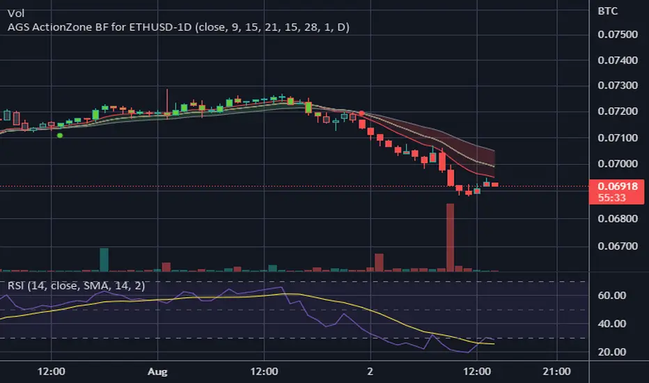
CDC ActionZone BF for ETHUSD-1D © PRoSkYNeT-EE
Based on improvements from "Kitti-Playbook Action Zone V.4.2.0.3 for Stock Market"
Based on improvements from "CDC Action Zone V3 2020 by piriya33"
Based on Triple MACD crossover between 9/15, 21/28, 15/28 for filter error signal (noise) from CDC ActionZone V3
MACDs generated from the execution of millions of times in the "Brute Force Algorithm" to backtest data from the past 5 years. ( 2017-08-21 to 2022-08-01 )
Released 2022-08-01
***** The indicator is used in the ETHUSD 1 Day period ONLY *****
Recommended Stop Loss : -4 % (execute stop Loss after candlestick has been closed)
Backtest Result ( Start $100 )
Winrate 63 % (Win:12, Loss:7, Total:19)
Live Days 1,806 days
B : Buy
S : Sell
SL : Stop Loss
2022-07-19 07 - 1,542 : B 6.971 ETH
2022-04-13 07 - 3,118 : S 8.98 % $10,750 12,7,19 63 %
2022-03-20 07 - 2,861 : B 3.448 ETH
2021-12-03 07 - 4,216 : SL -8.94 % $9,864 11,7,18 61 %
2021-11-30 07 - 4,630 : B 2.340 ETH
2021-11-18 07 - 3,997 : S 13.71 % $10,832 11,6,17 65 %
2021-10-05 07 - 3,515 : B 2.710 ETH
2021-09-20 07 - 2,977 : S 29.38 % $9,526 10,6,16 63 %
2021-07-28 07 - 2,301 : B 3.200 ETH
2021-05-20 07 - 2,769 : S 50.49 % $7,363 9,6,15 60 %
2021-03-30 07 - 1,840 : B 2.659 ETH
2021-03-22 07 - 1,681 : SL -8.29 % $4,893 8,6,14 57 %
2021-03-08 07 - 1,833 : B 2.911 ETH
2021-02-26 07 - 1,445 : S 279.27 % $5,335 8,5,13 62 %
2020-10-13 07 - 381 : B 3.692 ETH
2020-09-05 07 - 335 : S 38.43 % $1,407 7,5,12 58 %
2020-07-06 07 - 242 : B 4.199 ETH
2020-06-27 07 - 221 : S 28.49 % $1,016 6,5,11 55 %
2020-04-16 07 - 172 : B 4.598 ETH
2020-02-29 07 - 217 : S 47.62 % $791 5,5,10 50 %
2020-01-12 07 - 147 : B 3.644 ETH
2019-11-18 07 - 178 : S -2.73 % $536 4,5,9 44 %
2019-11-01 07 - 183 : B 3.010 ETH
2019-09-23 07 - 201 : SL -4.29 % $551 4,4,8 50 %
2019-09-18 07 - 210 : B 2.740 ETH
2019-07-12 07 - 275 : S 63.69 % $575 4,3,7 57 %
2019-05-03 07 - 168 : B 2.093 ETH
2019-04-28 07 - 158 : S 29.51 % $352 3,3,6 50 %
2019-02-15 07 - 122 : B 2.225 ETH
2019-01-10 07 - 125 : SL -6.02 % $271 2,3,5 40 %
2018-12-29 07 - 133 : B 2.172 ETH
2018-05-22 07 - 641 : S 5.95 % $289 2,2,4 50 %
2018-04-21 07 - 605 : B 0.451 ETH
2018-02-02 07 - 922 : S 197.42 % $273 1,2,3 33 %
2017-11-11 07 - 310 : B 0.296 ETH
2017-10-09 07 - 297 : SL -4.50 % $92 0,2,2 0 %
2017-10-07 07 - 311 : B 0.309 ETH
2017-08-22 07 - 310 : SL -4.02 % $96 0,1,1 0 %
2017-08-21 07 - 323 : B 0.310 ETH
[Delphi] 3EMA 3MA 3WMA Lin_RegCopyright by Delphi v3.0 04/07/2018
3EMA 3MA 3WMA Lin_Reg
Follow me for updates and strategies
20/06/2018 Added 3EMA 3MA 3WMA
04/07/2018 Added Linear Regression based on selected MA
04/07/2018 Added Enable option for every indicator

FNGAdataHighHigh prices for FNGA ETF (Dec 2018–May 2025)
The High prices for FNGA ETF (December 2018 – May 2025) represent the maximum trading price reached during each regular U.S. market session over the entire trading lifespan of this leveraged exchange-traded note. Originally issued under the ticker FNGU, and later rebranded as FNGA in March 2025 before its redemption, the fund was designed to deliver 3x daily leveraged exposure to the MicroSectors FANG+™ Index. This index focused on a concentrated group of large-cap technology and technology-enabled companies such as Facebook (Meta), Amazon, Apple, Netflix, and Google (Alphabet), along with a few other growth leaders.
The High price data from December 2018 through May 2025 is crucial for understanding how FNGA behaved during intraday trading sessions. Because FNGA was a daily resetting 3x leveraged product, its intraday highs often displayed extreme sensitivity to movements in the underlying FANG+™ stocks, resulting in sharp upward spikes during bullish days and pronounced volatility during broader market rallies.

[astropark] MACD, RSI+, AO, DMI, ADX, OBV, ADI//******************************************************************************
// Copyright by astropark v4.1.0
// MACD, RSI+, Awesome Oscillator, DMI, ADX, OBV, ADI
// 24/10/2018 Added RSI with Center line to have clear glue of current trend
// 10/12/2018 Added MACD
// 13/12/2018 Added multiplier for MACD in order to make it clearly visible over RSI graph
// 11/01/2019 Added Awesome Ascillator (AO)
// 11/01/2019 Added Directional Movement Index (DMI) with ADX
// 14/01/2019 Added On Balance Volume (OBV)
// 14/01/2019 Added Accelerator Decelerator Indicator (ADI)
//******************************************************************************
[astropark] MACD, RSI+, Awesome Oscillator, DMI, ADX, OBV//******************************************************************************
// Copyright by astropark v4.0.0
// MACD, RSI+, Awesome Oscillator, DMI, ADX, OBV
// 24/10/2018 Added RSI with Center line to have clear glue of current trend
// 10/12/2018 Added MACD
// 13/12/2018 Added multiplier for MACD in order to make it clearly visible over RSI graph
// 11/01/2019 Added Awesome Oscillator (AO)
// 11/01/2019 Added Directional Movement Index (DMI) with ADX
// 14/01/2019 Added On Balance Volume (OBV)
//******************************************************************************
[astropark] MACD, RSI+, Awesome Oscillator, DMI with ADX//******************************************************************************
// Copyright by astropark v3.1.0
// MACD, RSI+, Awesome Oscillator, DMI, ADX
// 24/10/2018 Added RSI with Center line to have clear glue of current trend
// 10/12/2018 Added MACD
// 13/12/2018 Added multiplier for MACD in order to make it clearly visible over RSI graph
// 11/01/2019 Added Awesome Ascillator (AO)
// 11/01/2019 Added Directional Movement Index (DMI) with ADX
//******************************************************************************
[astropark] MACD, RSI+, Awesome Oscillator//******************************************************************************
// Copyright by astropark v3.0.0
// MACD, RSI+, Awesome Oscillator
// 24/10/2018 Added RSI with Center line to have clear glue of current trend
// 10/12/2018 Added MACD
// 13/12/2018 Added multiplier for MACD in order to make it clearly visible over RSI graph
// 11/01/2019 Added Awesome Ascillator (AO)
//******************************************************************************

[astropark] MACD & RSI+//******************************************************************************
// Copyright by astropark v2.0
// MACD RSI+
// 24/10/2018 Added RSI with Center line to have clear glue of current trend
// 10/12/2018 Added MACD
// 13/12/2018 Added multiplier for MACD in order to make it clearly visible over RSI graph
//******************************************************************************

[Delphi] Power Tools OscillatorsFEATURES
- RSI
- Stochastic
//******************************************************************************
// Power Tools Oscillators
// Inner Version 1.0 04/12/2018
// Developer: iDelphi
//------------------------------------------------------------------------------
// 04/12/2018 Added RSI
// 04/12/2018 Added Stochastic
//******************************************************************************

[Delphi] 3EMA 3MA 3WMA Lin_Reg 3EMA 3MA 3WMA Lin_Reg
Follow me for updates and strategies
20/06/2018 Added 3EMA 3MA 3WMA
04/07/2018 Added Linear Regression based on selected MA
04/07/2018 Added Enable option for every indicator

[Delphi] 3EMA 3MA 3WMA Lin_RegCopyright by Delphi v3.0
3EMA 3MA 3WMA Lin_Reg
Follow me for updates and strategies
20/06/2018 Added 3EMA 3MA 3WMA
04/07/2018 Added Linear Regression based on selected MA
04/07/2018 Added Enable option for every indicator

[Delphi] RSI Pista CiclicaCopyright by Delphi v1.0 05/07/2018
RSI Pista Ciclica
Follow me for updates and strategies
05/07/2018 Added Pista Ciclica
05/07/2018 Added RSI

Day25RangeDay25Range(1) - Plot on the candle the 25% low range of the daily price. This helps to show when the current price is at or below the 25% price range of the day. Best when used with other indicators to show early wakening strength in price. On the attached chart, if you look at Jan 23, 2018 you will see a red candle that closed below the 25% mark of the trading day. For that day the 25% mark was at 38.66 and the close of the day was at 38.25 That indicators a potential start of a strong swing trade down. A second signal was given on Jan 25, 2018 when a red candle closed (37.25) below the 25% mark (38.08) again. Within the next few days a third weak indicator signaled on Jan 30,2018 with a close (35.88) below the Day25Range (37.46). price continued down from there for the next 4 days before starting to reverse. If the price closes below the 25% daily range as shown on the Day25Range(1) indicator, this could indicate a possible start of weakening in the price movement.