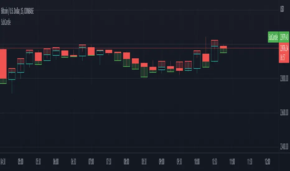
SubCandleI created this script as POC to handle specific cases where not having tick data on historical bars create repainting. Happy to share if this serves purpose for other coders.
What is the function of this script?
Script plots a sub-candle which is remainder of candle after forming the latest peak.
Higher body of Sub-candle refers to strong retracement of price from its latest peak. Color of the sub-candle defines the direction of retracement.
Higher wick of Sub-candle refers to higher push in the direction of original candle. Meaning, after price reaching its peak, price retraced but could not hold.
Here is a screenshot with explanation to visualise the concept:
Settings
There is only one setting which is number of backtest bars. Lower timeframe resolution which is used for calculating the Sub-candle uses this number to automatically calculate maximum possible lower timeframe so that all the required backtest windows are covered without having any issue.
We need to keep in mind that max available lower timeframe bars is 100,000. Hence, with 5000 backtest bars, lower timeframe resolution can be about 20 (100000/5000) times lesser than that of regular chart timeframe. We need to also keep in mind that minimum resolution available as part of security_lower_tf is 1 minute. Hence, it is not advisable to use this script for chart timeframes less than 15 mins.
Application
I have been facing this issue in pattern recognition scripts where patterns are formed using high/low prices but entry and targets are calculated based on the opposite side (low/high). It becomes tricky during extreme bars to identify entry conditions based on just the opposite peak because, the candle might have originated from it before identifying the pattern and might have never reached same peak after forming the pattern. Due to lack of tick data on historical bars, we cannot use close price to measure such conditions. This leads to repaint and few unexpected results. I am intending to use this method to overcome the issue up-to some extent.
在腳本中搜尋"wind+芯片行业+市盈率+财经数据"
Growth Stock Arbitrage Indicator [@PierceARK]This indicator takes advantage of the fact that when the 10 and 5 year Treasury Constant Maturity Minus Federal Funds rates (T10YFF/T5YFF) go down sharply, investors tend to rotate into stocks. This arbitrage works great for growth stocks, since growth stocks are higher beta by virtue of their lower market cap and more speculative nature in general. This script identifies the moving-average convergence/divergence of the average of the 10y and 5y treasury rates and then finds the variance of that macd line. By averaging that variance with the macdline's inverse, an analog output of treasury -> stock rotation can be identified. The upper and lower thresholds bring buy and sell windows into focus.

STD-Stepped Fast Cosine Transform Moving Average [Loxx]STD-Stepped Fast Cosine Transform Moving Average is an experimental moving average that uses Fast Cosine Transform to calculate a moving average. This indicator has standard deviation stepping in order to smooth the trend by weeding out low volatility movements.
What is the Discrete Cosine Transform?
A discrete cosine transform (DCT) expresses a finite sequence of data points in terms of a sum of cosine functions oscillating at different frequencies. The DCT, first proposed by Nasir Ahmed in 1972, is a widely used transformation technique in signal processing and data compression. It is used in most digital media, including digital images (such as JPEG and HEIF, where small high-frequency components can be discarded), digital video (such as MPEG and H.26x), digital audio (such as Dolby Digital, MP3 and AAC), digital television (such as SDTV, HDTV and VOD), digital radio (such as AAC+ and DAB+), and speech coding (such as AAC-LD, Siren and Opus). DCTs are also important to numerous other applications in science and engineering, such as digital signal processing, telecommunication devices, reducing network bandwidth usage, and spectral methods for the numerical solution of partial differential equations.
The use of cosine rather than sine functions is critical for compression, since it turns out (as described below) that fewer cosine functions are needed to approximate a typical signal, whereas for differential equations the cosines express a particular choice of boundary conditions. In particular, a DCT is a Fourier-related transform similar to the discrete Fourier transform (DFT), but using only real numbers. The DCTs are generally related to Fourier Series coefficients of a periodically and symmetrically extended sequence whereas DFTs are related to Fourier Series coefficients of only periodically extended sequences. DCTs are equivalent to DFTs of roughly twice the length, operating on real data with even symmetry (since the Fourier transform of a real and even function is real and even), whereas in some variants the input and/or output data are shifted by half a sample. There are eight standard DCT variants, of which four are common.
The most common variant of discrete cosine transform is the type-II DCT, which is often called simply "the DCT". This was the original DCT as first proposed by Ahmed. Its inverse, the type-III DCT, is correspondingly often called simply "the inverse DCT" or "the IDCT". Two related transforms are the discrete sine transform (DST), which is equivalent to a DFT of real and odd functions, and the modified discrete cosine transform (MDCT), which is based on a DCT of overlapping data. Multidimensional DCTs (MD DCTs) are developed to extend the concept of DCT to MD signals. There are several algorithms to compute MD DCT. A variety of fast algorithms have been developed to reduce the computational complexity of implementing DCT. One of these is the integer DCT (IntDCT), an integer approximation of the standard DCT, : ix, xiii, 1, 141–304 used in several ISO/IEC and ITU-T international standards.
Notable settings
windowper = period for calculation, restricted to powers of 2: "16", "32", "64", "128", "256", "512", "1024", "2048", this reason for this is FFT is an algorithm that computes DFT (Discrete Fourier Transform) in a fast way, generally in 𝑂(𝑁⋅log2(𝑁)) instead of 𝑂(𝑁2). To achieve this the input matrix has to be a power of 2 but many FFT algorithm can handle any size of input since the matrix can be zero-padded. For our purposes here, we stick to powers of 2 to keep this fast and neat. read more about this here: Cooley–Tukey FFT algorithm
smthper = smoothing count, this smoothing happens after the first FCT regular pass. this zeros out frequencies from the previously calculated values above SS count. the lower this number, the smoother the output, it works opposite from other smoothing periods
Included
Alerts
Signals
Loxx's Expanded Source Types
Additional reading
A Fast Computational Algorithm for the Discrete Cosine Transform by Chen et al.
Practical Fast 1-D DCT Algorithms With 11 Multiplications by Loeffler et al.
Cooley–Tukey FFT algorithm

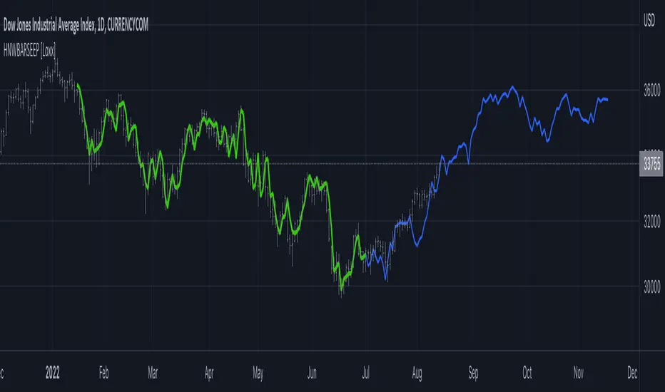
Helme-Nikias Weighted Burg AR-SE Extra. of Price [Loxx]Helme-Nikias Weighted Burg AR-SE Extra. of Price is an indicator that uses an autoregressive spectral estimation called the Weighted Burg Algorithm, but unlike the usual WB algo, this one uses Helme-Nikias weighting. This method is commonly used in speech modeling and speech prediction engines. This is a linear method of forecasting data. You'll notice that this method uses a different weighting calculation vs Weighted Burg method. This new weighting is the following:
w = math.pow(array.get(x, i - 1), 2), the squared lag of the source parameter
and
w += math.pow(array.get(x, i), 2), the sum of the squared source parameter
This take place of the rectangular, hamming and parabolic weighting used in the Weighted Burg method
Also, this method includes Levinson–Durbin algorithm. as was already discussed previously in the following indicator:
Levinson-Durbin Autocorrelation Extrapolation of Price
What is Helme-Nikias Weighted Burg Autoregressive Spectral Estimate Extrapolation of price?
In this paper a new stable modification of the weighted Burg technique for autoregressive (AR) spectral estimation is introduced based on data-adaptive weights that are proportional to the common power of the forward and backward AR process realizations. It is shown that AR spectra of short length sinusoidal signals generated by the new approach do not exhibit phase dependence or line-splitting. Further, it is demonstrated that improvements in resolution may be so obtained relative to other weighted Burg algorithms. The method suggested here is shown to resolve two closely-spaced peaks of dynamic range 24 dB whereas the modified Burg schemes employing rectangular, Hamming or "optimum" parabolic windows fail.
Data inputs
Source Settings: -Loxx's Expanded Source Types. You typically use "open" since open has already closed on the current active bar
LastBar - bar where to start the prediction
PastBars - how many bars back to model
LPOrder - order of linear prediction model; 0 to 1
FutBars - how many bars you want to forward predict
Things to know
Normally, a simple moving average is calculated on source data. I've expanded this to 38 different averaging methods using Loxx's Moving Avreages.
This indicator repaints
Further reading
A high-resolution modified Burg algorithm for spectral estimation
Related Indicators
Levinson-Durbin Autocorrelation Extrapolation of Price
Weighted Burg AR Spectral Estimate Extrapolation of Price
[blackcat] L1 Vitali Apirine HHs & LLs StochasticsLevel 1
Background
This indicator was originally formulated by Vitali Apirine for TASC - February 2016 Traders Tips.
Function
According to Vitali Apirine, his momentum indicator–based system HHLLS (higher high lower low stochastic) can help to spot emerging trends, define correction periods, and anticipate reversals. As with many indicators, HHLLS signals can also be generated by looking for divergences and crossovers. Because the HHLLS is an oscillator, it can also be used to identify overbought & oversold levels.
Remarks
I changed EMA or SMA into hanning windowing function to reduce lag issue.
colorful area is bearish power.
colorful solid thick line is bull power.
Feedbacks are appreciated.

No Climactic BarsThis script can be used to detect large candles, similiar to ATR, using the variance of a sliding windows and certain threshold.

NormalizedOscillatorsLibrary "NormalizedOscillators"
Collection of some common Oscillators. All are zero-mean and normalized to fit in the -1..1 range. Some are modified, so that the internal smoothing function could be configurable (for example, to enable Hann Windowing, that John F. Ehlers uses frequently). Some are modified for other reasons (see comments in the code), but never without a reason. This collection is neither encyclopaedic, nor reference, however I try to find the most correct implementation. Suggestions are welcome.
rsi2(upper, lower) RSI - second step
Parameters:
upper : Upwards momentum
lower : Downwards momentum
Returns: Oscillator value
Modified by Ehlers from Wilder's implementation to have a zero mean (oscillator from -1 to +1)
Originally: 100.0 - (100.0 / (1.0 + upper / lower))
Ignoring the 100 scale factor, we get: upper / (upper + lower)
Multiplying by two and subtracting 1, we get: (2 * upper) / (upper + lower) - 1 = (upper - lower) / (upper + lower)
rms(src, len) Root mean square (RMS)
Parameters:
src : Source series
len : Lookback period
Based on by John F. Ehlers implementation
ift(src) Inverse Fisher Transform
Parameters:
src : Source series
Returns: Normalized series
Based on by John F. Ehlers implementation
The input values have been multiplied by 2 (was "2*src", now "4*src") to force expansion - not compression
The inputs may be further modified, if needed
stoch(src, len) Stochastic
Parameters:
src : Source series
len : Lookback period
Returns: Oscillator series
ssstoch(src, len) Super Smooth Stochastic (part of MESA Stochastic) by John F. Ehlers
Parameters:
src : Source series
len : Lookback period
Returns: Oscillator series
Introduced in the January 2014 issue of Stocks and Commodities
This is not an implementation of MESA Stochastic, as it is based on Highpass filter not present in the function (but you can construct it)
This implementation is scaled by 0.95, so that Super Smoother does not exceed 1/-1
I do not know, if this the right way to fix this issue, but it works for now
netKendall(src, len) Noise Elimination Technology by John F. Ehlers
Parameters:
src : Source series
len : Lookback period
Returns: Oscillator series
Introduced in the December 2020 issue of Stocks and Commodities
Uses simplified Kendall correlation algorithm
Implementation by @QuantTherapy:
rsi(src, len, smooth) RSI
Parameters:
src : Source series
len : Lookback period
smooth : Internal smoothing algorithm
Returns: Oscillator series
vrsi(src, len, smooth) Volume-scaled RSI
Parameters:
src : Source series
len : Lookback period
smooth : Internal smoothing algorithm
Returns: Oscillator series
This is my own version of RSI. It scales price movements by the proportion of RMS of volume
mrsi(src, len, smooth) Momentum RSI
Parameters:
src : Source series
len : Lookback period
smooth : Internal smoothing algorithm
Returns: Oscillator series
Inspired by RocketRSI by John F. Ehlers (Stocks and Commodities, May 2018)
rrsi(src, len, smooth) Rocket RSI
Parameters:
src : Source series
len : Lookback period
smooth : Internal smoothing algorithm
Returns: Oscillator series
Inspired by RocketRSI by John F. Ehlers (Stocks and Commodities, May 2018)
Does not include Fisher Transform of the original implementation, as the output must be normalized
Does not include momentum smoothing length configuration, so always assumes half the lookback length
mfi(src, len, smooth) Money Flow Index
Parameters:
src : Source series
len : Lookback period
smooth : Internal smoothing algorithm
Returns: Oscillator series
lrsi(src, in_gamma, len) Laguerre RSI by John F. Ehlers
Parameters:
src : Source series
in_gamma : Damping factor (default is -1 to generate from len)
len : Lookback period (alternatively, if gamma is not set)
Returns: Oscillator series
The original implementation is with gamma. As it is impossible to collect gamma in my system, where the only user input is length,
an alternative calculation is included, where gamma is set by dividing len by 30. Maybe different calculation would be better?
fe(len) Choppiness Index or Fractal Energy
Parameters:
len : Lookback period
Returns: Oscillator series
The Choppiness Index (CHOP) was created by E. W. Dreiss
This indicator is sometimes called Fractal Energy
er(src, len) Efficiency ratio
Parameters:
src : Source series
len : Lookback period
Returns: Oscillator series
Based on Kaufman Adaptive Moving Average calculation
This is the correct Efficiency ratio calculation, and most other implementations are wrong:
the number of bar differences is 1 less than the length, otherwise we are adding the change outside of the measured range!
For reference, see Stocks and Commodities June 1995
dmi(len, smooth) Directional Movement Index
Parameters:
len : Lookback period
smooth : Internal smoothing algorithm
Returns: Oscillator series
Based on the original Tradingview algorithm
Modified with inspiration from John F. Ehlers DMH (but not implementing the DMH algorithm!)
Only ADX is returned
Rescaled to fit -1 to +1
Unlike most oscillators, there is no src parameter as DMI works directly with high and low values
fdmi(len, smooth) Fast Directional Movement Index
Parameters:
len : Lookback period
smooth : Internal smoothing algorithm
Returns: Oscillator series
Same as DMI, but without secondary smoothing. Can be smoothed later. Instead, +DM and -DM smoothing can be configured
doOsc(type, src, len, smooth) Execute a particular Oscillator from the list
Parameters:
type : Oscillator type to use
src : Source series
len : Lookback period
smooth : Internal smoothing algorithm
Returns: Oscillator series
Chande Momentum Oscillator (CMO) is RSI without smoothing. No idea, why some authors use different calculations
LRSI with Fractal Energy is a combo oscillator that uses Fractal Energy to tune LRSI gamma, as seen here: www.prorealcode.com
doPostfilter(type, src, len) Execute a particular Oscillator Postfilter from the list
Parameters:
type : Oscillator type to use
src : Source series
len : Lookback period
Returns: Oscillator series

Directional Movement w/Hann Slope Change SignalModified version of
Presented here is code for the "Directional Movement w/Hann" indicator originally conceived by John Ehlers. The code is also published in the December 2021 issue of Trader's Tips by Technical Analysis of Stocks & Commodities (TASC) magazine.
John Ehlers is continuing to revamp old indictors with Hann windowing. The original script uses zero line cross to signal buy/sell in this modified version buy/sell is signaled based on slope change, where signal is generated on with previous value is greater/less than current value
If current > previous = buy and if current < previous = sell

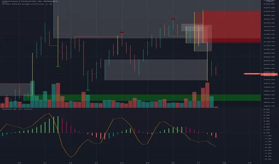
MAD indicator Enchanced (MADH, inspired by J.Ehlers)This oscillator was inspired by the recent J. Ehler's article (Stocks & Commodities V. 39:11 (24–26): The MAD Indicator, Enhanced by John F. Ehlers). Basically, it shows the difference between two move averages, an "enhancement" made by the author in the last version comes down to replacement SMA to a weighted average that uses Hann windowing. I took the liberty to add colors, ROC line (well, you know, no shorts when ROC's negative and no long's when positive, etc), and optional usage of PVT (price-volume trend) as the source (instead of just price).
[blackcat] L2 Ehlers Adaptive Jon Andersen R-Squared IndicatorLevel: 2
Background
@pips_v1 has proposed an interesting idea that is it possible to code an "Adaptive Jon Andersen R-Squared Indicator" where the length is determined by DCPeriod as calculated in Ehlers Sine Wave Indicator? I agree with him and starting to construct this indicator. After a study, I found "(blackcat) L2 Ehlers Autocorrelation Periodogram" script could be reused for this purpose because Ehlers Autocorrelation Periodogram is an ideal candidate to calculate the dominant cycle. On the other hand, there are two inputs for R-Squared indicator:
Length - number of bars to calculate moment correlation coefficient R
AvgLen - number of bars to calculate average R-square
I used Ehlers Autocorrelation Periodogram to produced a dynamic value of "Length" of R-Squared indicator and make it adaptive.
Function
One tool available in forecasting the trendiness of the breakout is the coefficient of determination (R-squared), a statistical measurement. The R-squared indicates linear strength between the security's price (the Y - axis) and time (the X - axis). The R-squared is the percentage of squared error that the linear regression can eliminate if it were used as the predictor instead of the mean value. If the R-squared were 0.99, then the linear regression would eliminate 99% of the error for prediction versus predicting closing prices using a simple moving average.
When the R-squared is at an extreme low, indicating that the mean is a better predictor than regression, it can only increase, indicating that the regression is becoming a better predictor than the mean. The opposite is true for extreme high values of the R-squared.
To make this indicator adaptive, the dominant cycle is extracted from the spectral estimate in the next block of code using a center-of-gravity ( CG ) algorithm. The CG algorithm measures the average center of two-dimensional objects. The algorithm computes the average period at which the powers are centered. That is the dominant cycle. The dominant cycle is a value that varies with time. The spectrum values vary between 0 and 1 after being normalized. These values are converted to colors. When the spectrum is greater than 0.5, the colors combine red and yellow, with yellow being the result when spectrum = 1 and red being the result when the spectrum = 0.5. When the spectrum is less than 0.5, the red saturation is decreased, with the result the color is black when spectrum = 0.
Construction of the autocorrelation periodogram starts with the autocorrelation function using the minimum three bars of averaging. The cyclic information is extracted using a discrete Fourier transform (DFT) of the autocorrelation results. This approach has at least four distinct advantages over other spectral estimation techniques. These are:
1. Rapid response. The spectral estimates start to form within a half-cycle period of their initiation.
2. Relative cyclic power as a function of time is estimated. The autocorrelation at all cycle periods can be low if there are no cycles present, for example, during a trend. Previous works treated the maximum cycle amplitude at each time bar equally.
3. The autocorrelation is constrained to be between minus one and plus one regardless of the period of the measured cycle period. This obviates the need to compensate for Spectral Dilation of the cycle amplitude as a function of the cycle period.
4. The resolution of the cyclic measurement is inherently high and is independent of any windowing function of the price data.
Key Signal
DC --> Ehlers dominant cycle.
AvgSqrR --> R-squared output of the indicator.
Remarks
This is a Level 2 free and open source indicator.
Feedbacks are appreciated.

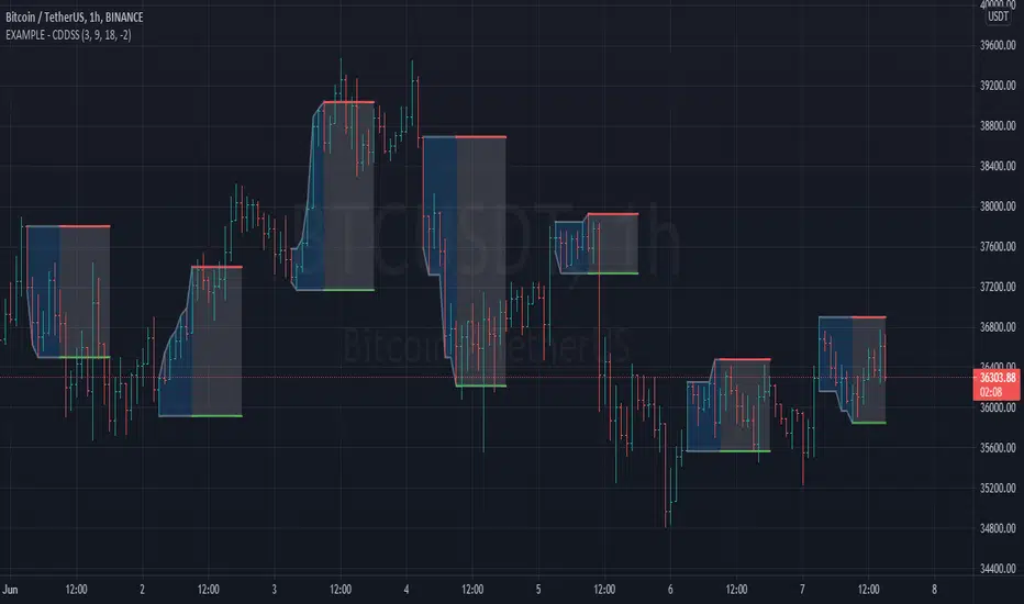
Example - Custom Defined Dual-State SessionThis script example aims to cover the following:
defining custom timeframe / session windows
gather a price range from the custom period ( high/low values )
create a secondary "holding" period through which to display the data collected from the initial session
simple method to shift times to re-align to preferred timezone
Articles and further reading:
www.investopedia.com - trading session
Reason for Study:
Educational purposes only.
Before considering writing this example I had seen multiple similar questions
asking how to go about creating custom timeframes or sessions, so it seemed
this might be a good topic to attempt to create a relatively generic example.
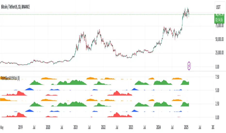
Pragmatic risk managementINTRO
The indicator is calculating multiple moving averages on the value of price change %. It then combines the normalized (via arctan function) values into a single normalized value (via simple average).
The total error from the center of gravity and the angle in which the error is accumulating represented by 4 waves:
BLUE = Good for chance for price to go up
GREEN = Good chance for price to continue going up
ORANGE = Good chance for price to go down
RED = Good chance for price to continue going down
A full cycle of ORANGE\RED\BLUE\GREEN colors will ideally lead to the exact same cycle, if not, try to understand why.
NOTICE-
This indicator is calculating large time-windows so It can be heavy on your device. Tested on PC browser only.
My visual setup:
1. Add two indicators on-top of each other and merge their scales (It will help out later).
2. Zoom out price chart to see the maximum possible data.
3. Set different colors for both indicators for simple visual seperation.
4. Choose 2 different values, one as high as possible and one as low as possible.
(Possible - the indicator remains effective at distinguishing the cycle).
Manual calibration:
0. Select a fixed chart resolution (2H resolution minimum recommended).
1. Change the "mul2" parameter in ranges between 4-15 .
2. Observe the "Turning points" of price movement. (Typically when RED\GREEN are about to switch.)
2. Perform a segmentation of time slices and find cycles. No need to be exact!
3. Draw a square on price movement at place and color as the dominant wave currently inside the indicator.
This procedure should lead to a full price segmentation with easier anchoring.
[blackcat] L2 Ehlers Autocorrelation PeriodogramLevel: 2
Background
John F. Ehlers introduced Autocorrelation Periodogram in his "Cycle Analytics for Traders" chapter 8 on 2013.
Function
Construction of the autocorrelation periodogram starts with the autocorrelation function using the minimum three bars of averaging. The cyclic information is extracted using a discrete Fourier transform (DFT) of the autocorrelation results. This approach has at least four distinct advantages over other spectral estimation techniques. These are:
1. Rapid response. The spectral estimates start to form within a half-cycle period of their initiation.
2. Relative cyclic power as a function of time is estimated. The autocorrelation at all cycle periods can be low if there are no cycles present, for example, during a trend. Previous works treated the maximum cycle amplitude at each time bar equally.
3. The autocorrelation is constrained to be between minus one and plus one regardless of the period of the measured cycle period. This obviates the need to compensate for Spectral Dilation of the cycle amplitude as a function of the cycle period.
4. The resolution of the cyclic measurement is inherently high and is independent of any windowing function of the price data.
The dominant cycle is extracted from the spectral estimate in the next block of code using a center-of-gravity (CG) algorithm. The CG algorithm measures the average center of two-dimensional objects. The algorithm computes the average period at which the powers are centered. That is the dominant cycle. The dominant cycle is a value that varies with time. The spectrum values vary between 0 and 1 after being normalized. These values are converted to colors. When the spectrum is greater than 0.5, the colors combine red and yellow, with yellow being the result when spectrum = 1 and red being the result when the spectrum = 0.5. When the spectrum is less than 0.5, the red saturation is decreased, with the result the color is black when spectrum = 0.
Key Signal
DominantCycle --> Dominant Cycle
Period --> Autocorrelation Periodogram Array
Pros and Cons
100% John F. Ehlers definition translation of original work, even variable names are the same. This help readers who would like to use pine to read his book. If you had read his works, then you will be quite familiar with my code style.
Remarks
The 49th script for Blackcat1402 John F. Ehlers Week publication.
Courtesy of @RicardoSantos for RGB functions.
Readme
In real life, I am a prolific inventor. I have successfully applied for more than 60 international and regional patents in the past 12 years. But in the past two years or so, I have tried to transfer my creativity to the development of trading strategies. Tradingview is the ideal platform for me. I am selecting and contributing some of the hundreds of scripts to publish in Tradingview community. Welcome everyone to interact with me to discuss these interesting pine scripts.
The scripts posted are categorized into 5 levels according to my efforts or manhours put into these works.
Level 1 : interesting script snippets or distinctive improvement from classic indicators or strategy. Level 1 scripts can usually appear in more complex indicators as a function module or element.
Level 2 : composite indicator/strategy. By selecting or combining several independent or dependent functions or sub indicators in proper way, the composite script exhibits a resonance phenomenon which can filter out noise or fake trading signal to enhance trading confidence level.
Level 3 : comprehensive indicator/strategy. They are simple trading systems based on my strategies. They are commonly containing several or all of entry signal, close signal, stop loss, take profit, re-entry, risk management, and position sizing techniques. Even some interesting fundamental and mass psychological aspects are incorporated.
Level 4 : script snippets or functions that do not disclose source code. Interesting element that can reveal market laws and work as raw material for indicators and strategies. If you find Level 1~2 scripts are helpful, Level 4 is a private version that took me far more efforts to develop.
Level 5 : indicator/strategy that do not disclose source code. private version of Level 3 script with my accumulated script processing skills or a large number of custom functions. I had a private function library built in past two years. Level 5 scripts use many of them to achieve private trading strategy.

predict lagUse the angle of multiple moving time windows to calculate the angular momentum vector across time. represent in a spectrum of frequencies\colors\transparency together with the accumulative "truth" (black)

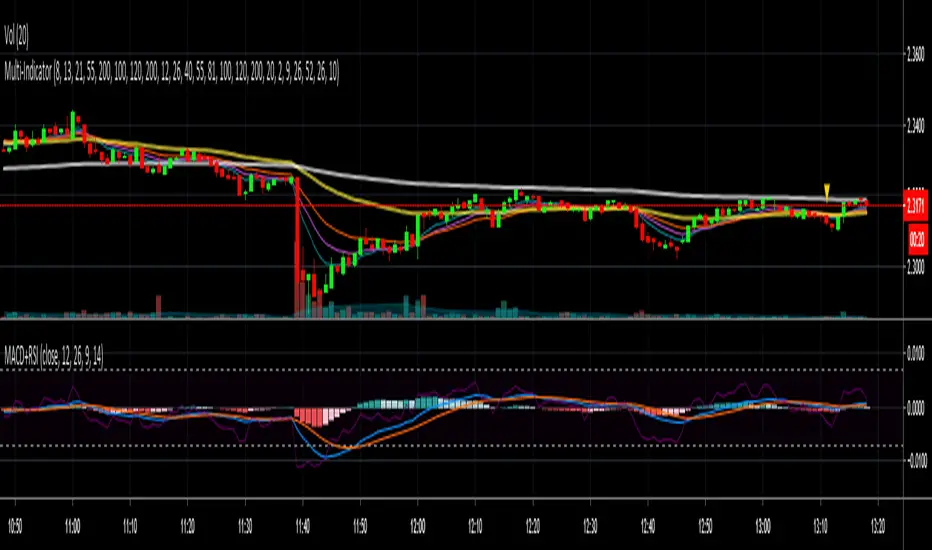
MACD + RSI togetheryou will have both MACD and RSI together in front of each other. best for tile windows or small monitors. enjoy
Better Bollinger Bands (now open source)General purpose Bollinger band indicator with a number of configuration options and some additional color-coded information. The main advantages of it over standard Bollinger bands are:
1) Better statistics:
* Uses volume weighted moving averages, variance, and standard deviation by default. The volume dependence can be disabled with a checkbox option, but generally makes it more responsive improves its ability to distinguish true outlier events from random variation.
* Lets you pick between different time windows (simple, sawtooth (WMA), exponential) in addition to the volume weighting, with appropriate Bessel corrections to make the estimators unbiased and to get consistent result for different weights.
* Has a checkbox option to use a linear regression in the band calculation if you don't want average momentum to be counted in the volatility. This turns the centerline into a last squares moving average, and the band width at each time step is given by the variance away from the regression line instead of from a moving average. Weights in the least squares regression are changed according to the other options. For tickers with a strong long-term trend this makes the bands track the price action more closely.
2) Geometric
* This does all calculations on log(price) instead of the prices themselves.
* Makes almost no difference in most cases, but gives better results on charts with strongly exponential behaviour that range between several orders of magnitude.
* Properly centered around price action on log plots.
* Will never annoy you by rescaling a log plot due to a negative lower band. The lower band is always positive for positive prices.
3) Some built in oscillators.
* This aims to reduce clutter by building in some other indicators into the band color scheme. You can pick between various momentum & RSI operators to color the center line and the bands, or leave the bands plain.
I've been using these bands myself for a few months & have been gradually adding functionality & polish. Feel free to comment, or to refer to me if you borrow any ideas.

FREE TRADINGVIEW FOR TIMEFRAMESWhen doing i.e the 3 minute timeframe turn on the closest timeframe available for you or the candles and wicks will be fucked up.
So if you're doing the 5 hour timeframe candles turn on the 4hr chart on your main chart.
To View the candles in full screen double click the windows with the candlesticks
If you don't have TradingView premium and want to look at custom timeframes you can use this.
For the ticker/coin/pair you want to show enter it like this:
For stocks, only the ticker i.e: MSFT, APPL
For Crypto, "Exchange:ticker" i.e: BITFINEX:BTCUSD, BINANCE:AGIBTC, BITMEX:ADAM19
When setting up the timeframe write i.e:
For minutes/hourly: 5, 240 (4 hour), 360 (6 hour)
For daily/weekly/monthly: 1D, 2W, 3M
When doing i.e the 3 minute timeframe turn on the closest timeframe available for you or the candles and wicks will be fucked up.
So if you're doing the 5 hour timeframe candles turn on the 4hr chart on your main chart.

Martingale Strategy Simulator [BackQuant]Martingale Strategy Simulator
Purpose
This indicator lets you study how a martingale-style position sizing rule interacts with a simple long or short trading signal. It computes an equity curve from bar-to-bar returns, adapts position size after losing streaks, caps exposure at a user limit, and summarizes risk with portfolio metrics. An optional Monte Carlo module projects possible future equity paths from your realized daily returns.
What a martingale is
A martingale sizing rule increases stake after losses and resets after a win. In its classical form from gambling, you double the bet after each loss so that a single win recovers all prior losses plus one unit of profit. In markets there is no fixed “even-money” payout and returns are multiplicative, so an exact recovery guarantee does not exist. The core idea is unchanged:
Lose one leg → increase next position size
Lose again → increase again
Win → reset to the base size
The expectation of your strategy still depends on the signal’s edge. Sizing does not create positive expectancy on its own. A martingale raises variance and tail risk by concentrating more capital as a losing streak develops.
What it plots
Equity – simulated portfolio equity including compounding
Buy & Hold – equity from holding the chart symbol for context
Optional helpers – last trade outcome, current streak length, current allocation fraction
Optional diagnostics – daily portfolio return, rolling drawdown, metrics table
Optional Monte Carlo probability cone – p5, p16, p50, p84, p95 aggregate bands
Model assumptions
Bar-close execution with no slippage or commissions
Shorting allowed and frictionless
No margin interest, borrow fees, or position limits
No intrabar moves or gaps within a bar (returns are close-to-close)
Sizing applies to equity fraction only and is capped by your setting
All results are hypothetical and for education only.
How the simulator applies it
1) Directional signal
You pick a simple directional rule that produces +1 for long or −1 for short each bar. Options include 100 HMA slope, RSI above or below 50, EMA or SMA crosses, CCI and other oscillators, ATR move, BB basis, and more. The stance is evaluated bar by bar. When the stance flips, the current trade ends and the next one starts.
2) Sizing after losses and wins
Position size is a fraction of equity:
Initial allocation – the starting fraction, for example 0.15 means 15 percent of equity
Increase after loss – multiply the next allocation by your factor after a losing leg, for example 2.00 to double
Reset after win – return to the initial allocation
Max allocation cap – hard ceiling to prevent runaway growth
At a high level the size after k consecutive losses is
alloc(k) = min( cap , base × factor^k ) .
In practice the simulator changes size only when a leg ends and its PnL is known.
3) Equity update
Let r_t = close_t / close_{t-1} − 1 be the symbol’s bar return, d_{t−1} ∈ {+1, −1} the prior bar stance, and a_{t−1} the prior bar allocation fraction. The simulator compounds:
eq_t = eq_{t−1} × (1 + a_{t−1} × d_{t−1} × r_t) .
This is bar-based and avoids intrabar lookahead. Costs, slippage, and borrowing costs are not modeled.
Why traders experiment with martingale sizing
Mean-reversion contexts – if the signal often snaps back after a string of losses, adding size near the tail of a move can pull the average entry closer to the turn
Behavioral or microstructure edges – some rules have modest edge but frequent small whipsaws; size escalation may shorten time-to-recovery when the edge manifests
Exploration and stress testing – studying the relationship between streaks, caps, and drawdowns is instructive even if you do not deploy martingale sizing live
Why martingale is dangerous
Martingale concentrates capital when the strategy is performing worst. The main risks are structural, not cosmetic:
Loss streaks are inevitable – even with a 55 percent win rate you should expect multi-loss runs. The probability of at least one k-loss streak in N trades rises quickly with N.
Size explodes geometrically – with factor 2.0 and base 10 percent, the sequence is 10, 20, 40, 80, 100 (capped) after five losses. Without a strict cap, required size becomes infeasible.
No fixed payout – in gambling, one win at even odds resets PnL. In markets, there is no guaranteed bounce nor fixed profit multiple. Trends can extend and gaps can skip levels.
Correlation of losses – losses cluster in trends and in volatility bursts. A martingale tends to be largest just when volatility is highest.
Margin and liquidity constraints – leverage limits, margin calls, position limits, and widening spreads can force liquidation before a mean reversion occurs.
Fat tails and regime shifts – assumptions of independent, Gaussian returns can understate tail risk. Structural breaks can keep the signal wrong for much longer than expected.
The simulator exposes these dynamics in the equity curve, Max Drawdown, VaR and CVaR, and via Monte Carlo sketches of forward uncertainty.
Interpreting losing streaks with numbers
A rough intuition: if your per-trade win probability is p and loss probability is q=1−p , the chance of a specific run of k consecutive losses is q^k . Over many trades, the chance that at least one k-loss run occurs grows with the number of opportunities. As a sanity check:
If p=0.55 , then q=0.45 . A 6-loss run has probability q^6 ≈ 0.008 on any six-trade window. Across hundreds of trades, a 6 to 8-loss run is not rare.
If your size factor is 1.5 and your base is 10 percent, after 8 losses the requested size is 10% × 1.5^8 ≈ 25.6% . With factor 2.0 it would try to be 10% × 2^8 = 256% but your cap will stop it. The equity curve will still wear the compounded drawdown from the sequence that led to the cap.
This is why the cap setting is central. It does not remove tail risk, but it prevents the sizing rule from demanding impossible positions
Note: The p and q math is illustrative. In live data the win rate and distribution can drift over time, so real streaks can be longer or shorter than the simple q^k intuition suggests..
Using the simulator productively
Parameter studies
Start with conservative settings. Increase one element at a time and watch how the equity, Max Drawdown, and CVaR respond.
Initial allocation – lower base reduces volatility and drawdowns across the board
Increase factor – set modestly above 1.0 if you want the effect at all; doubling is aggressive
Max cap – the most important brake; many users keep it between 20 and 50 percent
Signal selection
Keep sizing fixed and rotate signals to see how streak patterns differ. Trend-following signals tend to produce long wrong-way streaks in choppy ranges. Mean-reversion signals do the opposite. Martingale sizing interacts very differently with each.
Diagnostics to watch
Use the built-in metrics to quantify risk:
Max Drawdown – worst peak-to-trough equity loss
Sharpe and Sortino – volatility and downside-adjusted return
VaR 95 percent and CVaR – tail risk measures from the realized distribution
Alpha and Beta – relationship to your chosen benchmark
If you would like to check out the original performance metrics script with multiple assets with a better explanation on all metrics please see
Monte Carlo exploration
When enabled, the forecast draws many synthetic paths from your realized daily returns:
Choose a horizon and a number of runs
Review the bands: p5 to p95 for a wide risk envelope; p16 to p84 for a narrower range; p50 as the median path
Use the table to read the expected return over the horizon and the tail outcomes
Remember it is a sketch based on your recent distribution, not a predictor
Concrete examples
Example A: Modest martingale
Base 10 percent, factor 1.25, cap 40 percent, RSI>50 signal. You will see small escalations on 2 to 4 loss runs and frequent resets. The equity curve usually remains smooth unless the signal enters a prolonged wrong-way regime. Max DD may rise moderately versus fixed sizing.
Example B: Aggressive martingale
Base 15 percent, factor 2.0, cap 60 percent, EMA cross signal. The curve can look stellar during favorable regimes, then a single extended streak pushes allocation to the cap, and a few more losses drive deep drawdown. CVaR and Max DD jump sharply. This is a textbook case of high tail risk.
Strengths
Bar-by-bar, transparent computation of equity from stance and size
Explicit handling of wins, losses, streaks, and caps
Portable signal inputs so you can A–B test ideas quickly
Risk diagnostics and forward uncertainty visualization in one place
Example, Rolling Max Drawdown
Limitations and important notes
Martingale sizing can escalate drawdowns rapidly. The cap limits position size but not the possibility of extended adverse runs.
No commissions, slippage, margin interest, borrow costs, or liquidity limits are modeled.
Signals are evaluated on closes. Real execution and fills will differ.
Monte Carlo assumes independent draws from your recent return distribution. Markets often have serial correlation, fat tails, and regime changes.
All results are hypothetical. Use this as an educational tool, not a production risk engine.
Practical tips
Prefer gentle factors such as 1.1 to 1.3. Doubling is usually excessive outside of toy examples.
Keep a strict cap. Many users cap between 20 and 40 percent of equity per leg.
Stress test with different start dates and subperiods. Long flat or trending regimes are where martingale weaknesses appear.
Compare to an anti-martingale (increase after wins, cut after losses) to understand the other side of the trade-off.
If you deploy sizing live, add external guardrails such as a daily loss cut, volatility filters, and a global max drawdown stop.
Settings recap
Backtest start date and initial capital
Initial allocation, increase-after-loss factor, max allocation cap
Signal source selector
Trading days per year and risk-free rate
Benchmark symbol for Alpha and Beta
UI toggles for equity, buy and hold, labels, metrics, PnL, and drawdown
Monte Carlo controls for enable, runs, horizon, and result table
Final thoughts
A martingale is not a free lunch. It is a way to tilt capital allocation toward losing streaks. If the signal has a real edge and mean reversion is common, careful and capped escalation can reduce time-to-recovery. If the signal lacks edge or regimes shift, the same rule can magnify losses at the worst possible moment. This simulator makes those trade-offs visible so you can calibrate parameters, understand tail risk, and decide whether the approach belongs anywhere in your research workflow.

Live Market - Performance MonitorLive Market — Performance Monitor
Study material (no code) — step-by-step training guide for learners
________________________________________
1) What this tool is — short overview
This indicator is a live market performance monitor designed for learning. It scans price, volume and volatility, detects order blocks and trendline events, applies filters (volume & ATR), generates trade signals (BUY/SELL), creates simple TP/SL trade management, and renders a compact dashboard summarizing market state, risk and performance metrics.
Use it to learn how multi-factor signals are constructed, how Greeks-style sensitivity is replaced by volatility/ATR reasoning, and how a live dashboard helps monitor trade quality.
________________________________________
2) Quick start — how a learner uses it (step-by-step)
1. Add the indicator to a chart (any ticker / timeframe).
2. Open inputs and review the main groups: Order Block, Trendline, Signal Filters, Display.
3. Start with defaults (OB periods ≈ 7, ATR multiplier 0.5, volume threshold 1.2) and observe the dashboard on the last bar.
4. Walk the chart back in time (use the last-bar update behavior) and watch how signals, order blocks, trendlines, and the performance counters change.
5. Run the hands-on labs below to build intuition.
________________________________________
3) Main configurable inputs (what you can tweak)
• Order Block Relevant Periods (default ~7): number of consecutive candles used to define an order block.
• Min. Percent Move for Valid OB (threshold): minimum percent move required for a valid order block.
• Number of OB Channels: how many past order block lines to keep visible.
• Trendline Period (tl_period): pivot lookback for detecting highs/lows used to draw trendlines.
• Use Wicks for Trendlines: whether pivot uses wicks or body.
• Extension Bars: how far trendlines are projected forward.
• Use Volume Filter + Volume Threshold Multiplier (e.g., 1.2): requires volume to be greater than multiplier × average volume.
• Use ATR Filter + ATR Multiplier: require bar range > ATR × multiplier to filter noise.
• Show Targets / Table settings / Colors for visualization.
________________________________________
4) Core building blocks — what the script computes (plain language)
Price & trend:
• Spot / LTP: current close price.
• EMA 9 / 21 / 50: fast, medium, slow moving averages to define short/medium trend.
o trend_bullish: EMA9 > EMA21 > EMA50
o trend_bearish: EMA9 < EMA21 < EMA50
o trend_neutral: otherwise
Volatility & noise:
• ATR (14): average true range used for dynamic target and filter sizing.
• dynamic_zone = ATR × atr_multiplier: minimum bar range required for meaningful move.
• Annualized volatility: stdev of price changes × sqrt(252) × 100 — used to classify volatility (HIGH/MEDIUM/LOW).
Momentum & oscillators:
• RSI 14: overbought/oversold indicator (thresholds 70/30).
• MACD: EMA(12)-EMA(26) and a 9-period signal line; histogram used for momentum direction and strength.
• Momentum (ta.mom 10): raw momentum over 10 bars.
Mean reversion / band context:
• Bollinger Bands (20, 2σ): upper, mid, lower.
o price_position measures where price sits inside the band range as 0–100.
Volume metrics:
• avg_volume = SMA(volume, 20) and volume_spike = volume > avg_volume × volume_threshold
o volume_ratio = volume / avg_volume
Support & Resistance:
• support_level = lowest low over 20 bars
• resistance_level = highest high over 20 bars
• current_position = percent of price between support & resistance (0–100)
________________________________________
5) Order Block detection — concept & logic
What it tries to find: a bar (the base) followed by N candles in the opposite direction (a classical order block setup), with a minimum % move to qualify. The script records the high/low of the base candle, averages them, and plots those levels as OB channels.
How learners should think about it (conceptual):
1. An order block is a signature area where institutions (theory) left liquidity — often seen as a large bar followed by a sequence of directional candles.
2. This indicator uses a configurable number of subsequent candles to confirm that the pattern exists.
3. When found, it stores and displays the base candle’s high/low area so students can see how price later reacts to those zones.
Implementation note for learners: the tool keeps a limited history of OB lines (ob_channels). When new OBs exceed the count, the oldest lines are removed — good practice to avoid clutter.
________________________________________
6) Trendline detection — idea & interpretation
• The script finds pivot highs and lows using a symmetric lookback (tl_period and half that as right/left).
• It then computes a trendline slope from successive pivots and projects the line forward (extension_bars).
• Break detection: Resistance break = close crosses above the projected resistance line; Support break = close crosses below projected support.
Learning tip: trendlines here are computed from pivot points and time. Watch how changing tl_period (bigger = smoother, fewer pivots) alters the trendlines and break signals.
________________________________________
7) Signal generation & filters — step-by-step
1. Primary triggers:
o Bullish trigger: order block bullish OR resistance trendline break.
o Bearish trigger: bearish order block OR support trendline break.
2. Filters applied (both must pass unless disabled):
o Volume filter: volume must be > avg_volume × volume_threshold.
o ATR filter: bar range (high-low) must exceed ATR × atr_multiplier.
o Not in an existing trade: new trades only start if trade_active is false.
3. Trend confirmation:
o The primary trigger is only confirmed if trend is bullish/neutral for buys or bearish/neutral for sells (EMA alignment).
4. Result:
o When confirmed, a long or short trade is activated with TP/SL calculated from ATR multiples.
________________________________________
8) Trade management — what the tool does after a signal
• Entry management: the script marks a trade as trade_active and sets long_trade or short_trade flags.
• TP & SL rules:
o Long: TP = high + 2×ATR ; SL = low − 1×ATR
o Short: TP = low − 2×ATR ; SL = high + 1×ATR
• Monitoring & exit:
o A trade closes when price reaches TP or SL.
o When TP/SL hit, the indicator updates win_count and total_pnl using a very simple calculation (difference between TP/SL and previous close).
o Visual lines/labels are drawn for TP and updated as the trade runs.
Important learner notes:
• The script does not store a true entry price (it uses close in its P&L math), so PnL is an approximation — treat this as a learning proxy, not a position accounting system.
• There’s no sizing, slippage, or fee accounted — students must manually factor these when translating to real trades.
• This indicator is not a backtesting strategy; strategy.* functions would be needed for rigorous backtest results.
________________________________________
9) Signal strength & helper utilities
• Signal strength is a composite score (0–100) made up of four signals worth 25 points each:
1. RSI extreme (overbought/oversold) → 25
2. Volume spike → 25
3. MACD histogram magnitude increasing → 25
4. Trend existence (bull or bear) → 25
• Progress bars (text glyphs) are used to visually show RSI and signal strength on the table.
Learning point: composite scoring is a way to combine orthogonal signals — study how changing weights changes outcomes.
________________________________________
10) Dashboard — how to read each section (walkthrough)
The dashboard is split into sections; here's how to interpret them:
1. Market Overview
o LTP / Change%: immediate price & daily % change.
2. RSI & MACD
o RSI value plus progress bar (overbought 70 / oversold 30).
o MACD histogram sign indicates bullish/bearish momentum.
3. Volume Analysis
o Volume ratio (current / average) and whether there’s a spike.
4. Order Block Status
o Buy OB / Sell OB: the average base price of detected order blocks or “No Signal.”
5. Signal Status
o 🔼 BUY or 🔽 SELL if confirmed, or ⚪ WAIT.
o No-trade vs Active indicator summarizing market readiness.
6. Trend Analysis
o Trend direction (from EMAs), market sentiment score (composite), volatility level and band/position metrics.
7. Performance
o Win Rate = wins / signals (percentage)
o Total PnL = cumulative PnL (approximate)
o Bull / Bear Volume = accumulated volumes attributable to signals
8. Support & Resistance
o 20-bar highest/lowest — use as nearby reference points.
9. Risk & R:R
o Risk Level from ATR/price as a percent.
o R:R Ratio computed from TP/SL if a trade is active.
10. Signal Strength & Active Trade Status
• Numeric strength + progress bar and whether a trade is currently active with TP/SL display.
________________________________________
11) Alerts — what will notify you
The indicator includes pre-built alert triggers for:
• Bullish confirmed signal
• Bearish confirmed signal
• TP hit (long/short)
• SL hit (long/short)
• No-trade zone
• High signal strength (score > 75%)
Training use: enable alerts during a replay session to be notified when the indicator would have signalled.
________________________________________
12) Labs — hands-on exercises for learners (step-by-step)
Lab A — Order Block recognition
1. Pick a 15–30 minute timeframe on a liquid ticker.
2. Use default OB periods (7). Mark each time the dashboard shows a Buy/Sell OB.
3. Manually inspect the chart at the base candle and the following sequence — draw the OB zone by hand and watch later price reactions to it.
4. Repeat with OB periods 5 and 10; note stability vs noise.
Lab B — Trendline break confirmation
1. Increase trendline period (e.g., 20), watch trendlines form from pivots.
2. When a resistance break is flagged, compare with MACD & volume: was momentum aligned?
3. Note false breaks vs confirmed moves — change extension_bars to see projection effects.
Lab C — Filter sensitivity
1. Toggle Use Volume Filter off, and record the number and quality of signals in a 2-day window.
2. Re-enable volume filter and change threshold from 1.2 → 1.6; note how many low-quality signals are filtered out.
Lab D — Trade management simulation
1. For each signalled trade, record the time, close entry approximation, TP, SL, and eventual hit/miss.
2. Compute actual PnL if you had entered at the open of the next bar to compare with the script’s PnL math.
3. Tabulate win rate and average R:R.
Lab E — Performance review & improvement
1. Build a spreadsheet of signals over 30–90 periods with columns: Date, Signal type, Entry price (real), TP, SL, Exit, PnL, Notes.
2. Analyze which filters or indicators contributed most to winners vs losers and adjust weights.
________________________________________
13) Common pitfalls, assumptions & implementation notes (things to watch)
• P&L simplification: total_pnl uses close as a proxy entry price. Real entry/exit prices and slippage are not recorded — so PnL is approximate.
• No position sizing or money management: the script doesn’t compute position size from equity or risk percent.
• Signal confirmation logic: composite "signal_strength" is a simple 4×25 point scheme — explore different weights or additional signals.
• Order block detection nuance: the script defines the base candle and checks the subsequent sequence. Be sure to verify whether the intended candle direction (base being bullish vs bearish) aligns with academic/your trading definition — read the code carefully and test.
• Trendline slope over time: slope is computed using timestamps; small differences may make lines sensitive on very short timeframes — using bar_index differences is usually more stable.
• Not a true backtester: to evaluate performance statistically you must transform the logic into a strategy script that places hypothetical orders and records exact entry/exit prices.
________________________________________
14) Suggested improvements for advanced learners
• Record true entry price & timestamp for accurate PnL.
• Add position sizing: risk % per trade using SL distance and account size.
• Convert to strategy. (Pine Strategy)* to run formal backtests with equity curves, drawdowns, and metrics (Sharpe, Sortino).
• Log trades to an external spreadsheet (via alerts + webhook) for offline analysis.
• Add statistics: average win/loss, expectancy, max drawdown.
• Add additional filters: news time blackout, market session filters, multi-timeframe confirmation.
• Improve OB detection: combine wick/body, volume spike at base bar, and liquidity sweep detection.
________________________________________
15) Glossary — quick definitions
• ATR (Average True Range): measure of typical range; used to size targets and stops.
• EMA (Exponential Moving Average): trend smoothing giving more weight to recent prices.
• RSI (Relative Strength Index): momentum oscillator; >70 overbought, <30 oversold.
• MACD: momentum oscillator using difference of two EMAs.
• Bollinger Bands: volatility bands around SMA.
• Order Block: a base candle area with subsequent confirmation candles; a zone of institutional interest (learning model).
• Pivot High/Low: local turning point defined by candles on both sides.
• Signal Strength: combined score from multiple indicators.
• Win Rate: proportion of signals that hit TP vs total signals.
• R:R (Risk:Reward): ratio of potential reward (TP distance) to risk (entry to SL).
________________________________________
16) Limitations & assumptions (be explicit)
• This is an indicator for learning — not a trading robot or broker connection.
• No slippage, fees, commissions or tie-in to real orders are considered.
• The logic is heuristic (rule-of-thumb), not a guarantee of performance.
• Results are sensitive to timeframe, market liquidity, and parameter choices.
________________________________________
17) Practical classroom / study plan (4 sessions)
• Session 1 — Foundations: Understand EMAs, ATR, RSI, MACD, Bollinger Bands. Run the indicator and watch how these numbers change on a single day.
• Session 2 — Zones & Filters: Study order blocks and trendlines. Test volume & ATR filters and note changes in false signals.
• Session 3 — Simulated trading: Manually track 20 signals, compute real PnL and compare to the dashboard.
• Session 4 — Improvement plan: Propose changes (e.g., better PnL accounting, alternative OB rule) and test their impact.
________________________________________
18) Quick reference checklist for each signal
1. Was an order block or trendline break detected? (primary trigger)
2. Did volume meet threshold? (filter)
3. Did ATR filter (bar size) show a real move? (filter)
4. Was trend aligned (EMA 9/21/50)? (confirmation)
5. Signal confirmed → mark entry approximation, TP, SL.
6. Monitor dashboard (Signal Strength, Volatility, No-trade zone, R:R).
7. After exit, log real entry/exit, compute actual PnL, update spreadsheet.
________________________________________
19) Educational caveat & final note
This tool is built for training and analysis: it helps you see how common technical building blocks combine into trade ideas, but it is not a trading recommendation. Use it to develop judgment, to test hypotheses, and to design robust systems with proper backtesting and risk control before risking capital.
________________________________________
20) Disclaimer (must include)
Training & Educational Only — This material and the indicator are provided for educational purposes only. Nothing here is investment advice or a solicitation to buy or sell financial instruments. Past simulated or historical performance does not predict future results. Always perform full backtesting and risk management, and consider seeking advice from a qualified financial professional before trading with real capital.
________________________________________

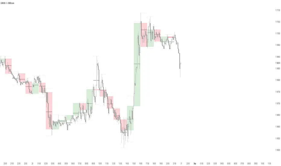
B A N K $ - HTF Candle Boxes (Power of 3)This indicator allows you to visualise the HTF candles on the LTF's, this is useful for using the Power of 3 / Accumulation, Manipulation & Distribution concepts.
By default, the HTF interval is set to 1h, this means that an outline will be created around the LTF candles that are within that 1h window. (i.e from 13:00-14:00 etc).
Features
HTF Interval Selector - this allows the user to customise which HTF interval to use
Candle Boxes - this outlines the full outer perimeter of the relevant candles
Include Body - this highlights the distance between the candle Open & Close
Show MidLine
Additional Settings
Hide Side Lines - this will only draw the Top & Bottom lines
Extend Lines to Current Candle - most recent Top & Bottom lines will extend to current price
Draw Lines from Exact Candle - this makes the most recent candle lines cleaner
I personally use this indicator to outline the most recent 3 1h candles to make it easier to identify sweeps & reversals however there is additional functionality to allow the user to customise the indicator to their preference.
Quantum Edge Scalper - Adaptive Precision Trading [KedArc Quant]Strategy Overview
Quantum Edge Scalper is a multi-regime intraday strategy engineered for adaptability across equities. It fuses EMA trend & slope, RSI sanity checks, ATR-based volatility gating, and candle-shape filters. Regime detection (ATR%% z-score) tunes thresholds on-the-fly, while an optional OSS — Oversold Short Override captures late-session breakdowns. Robust day-level controls include trade caps, cooldowns, and loss-streak stops. A compact panel summarizes live session stats.
Key Features
• Preset modes: Aggressive / Aggressive+ / Conservative / Hybrid / Custom.
• EMA Fast/Slow trend filter + EMA-separation slope gate.
• ATR volatility floor (percent-of-price) to avoid dead markets.
• Candle-shape and wick-ratio filters to curb false breakouts.
• Regime adaptation using ATR% z-score (HIGH / LOW / NEUTRAL).
• Hybrid+ LOW-regime extras: tighter SL, adaptive TP, mid-session pause, loss-streak blocker.
• OSS (Oversold Short Override): validators for micro-pullback, range expansion, structure break, and time window.
• Daily caps & loss-streak protection; cooldown management post wins/losses.
• Clean summary labels + compare panel; optional debug labels.

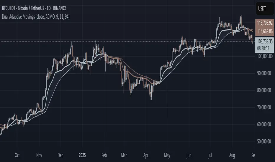
Dual Adaptive Movings### Dual Adaptive Movings
By Gurjit Singh
A dual-layer adaptive moving average system that adjusts its responsiveness dynamically using market-derived factors (CMO, RSI, Fractal Roughness, or Stochastic Acceleration). It plots:
* Primary Adaptive MA (MA): Fast, reacts to changes in volatility/momentum.
* Following Adaptive MA (FAMA): A smoother, half-alpha version for trend confirmation.
Instead of fixed smoothing, it adapts dynamically using one of four methods:
* ACMO: Adaptive CMO (momentum)
* ARSI: Adaptive RSI (relative strength)
* FRMA: Fractal Roughness (volatility + fractal dimension)
* ASTA: Adaptive Stochastic Acceleration (%K acceleration)
### ⚙️ Inputs & Options
* Source: Price input (default: close).
* Moving (Type): ACMO, ARSI, FRMA, ASTA.
* MA Length (Primary): Core adaptive window.
* Following (FAMA) Length: Optional; can match MA length.
* Use Wilder’s: Toggles Wilder vs EMA-style smoothing.
* Colors & Fill: Bullish/Bearish tones with transparency control.
### 🔑 How to Use
1. Identify Trend:
* When MA > FAMA → Bullish (fills bullish color).
* When MA < FAMA → Bearish (fills bearish color).
2. Crossovers:
* MA crosses above FAMA → Bullish signal 🐂
* MA crosses below FAMA → Bearish signal 🐻
3. Adaptive Edge:
* Select method (ACMO/ARSI/FRMA/ASTA) depending on whether you want sensitivity to momentum, strength, volatility, or acceleration.
4. Alerts:
* Built-in alerts trigger on crossovers.
### 💡 Tips
* Wilder’s smoothing is gentler than EMA, reducing whipsaws in sideways conditions.
* ACMO and ARSI are best for momentum-driven directional markets, but may false-signal in ranges.
* FRMA and ASTA excels in choppy markets where volatility clusters.
👉 In short: Dual Adaptive Movings adapts moving averages to the market’s own behavior, smoothing noise yet staying responsive. Crossovers mark possible trend shifts, while color fills highlight bias.
Trend by ΔMA + Double ZigZag + EMA/WMA Bands by KidevThis script is a multi-tool trend and structure analyzer combining moving average slope confirmation, double zigzag swing mapping, and dynamic EMA/WMA trend bands — all in one overlay indicator.
🔹 Key Features:
ΔMA Trend Detection
Detects trend shifts using the slope of a chosen moving average (SMA, EMA, WMA, RMA, HMA).
Confirms uptrend/downtrend only after a user-defined confirmation window.
Draws color-coded MA line (green = uptrend, red = downtrend, gray = sideways).
Optional arrows for trend change entries.
Alerts for confirmed trend shifts.
Double ZigZag Swing Analysis
Two customizable ZigZag layers with independent lookback periods.
Optional swing labels (HH, HL, LH, LL) to track market structure.
Full control over line style, width, and colors for each ZigZag.
EMA Band (96 default)
Plots a dynamic EMA channel (High, HLC3, Low).
Visual band highlights volatility and trend zones.
Adjustable fill color and transparency.
Weighted Moving Average (WMA 96)
Clean trend-following baseline.
Adjustable source, length, and color.
Background Highlight
Toggleable background shading for bullish / bearish / sideways conditions.
Fully customizable colors and transparency.
Helps visually separate market phases at a glance.
Note:
ZigZag repainting is inherent by design (future swings refine past points). Use it as a structural guide, not as a standalone signal.
