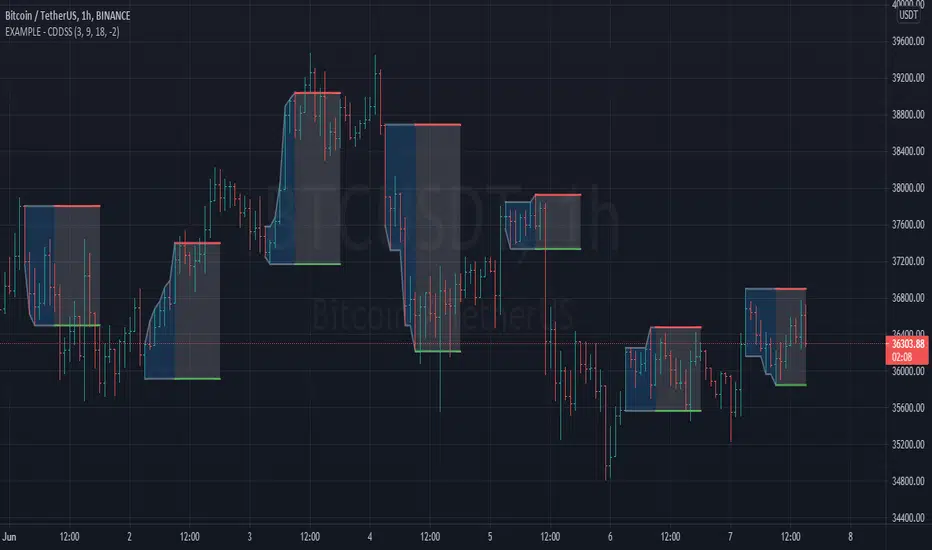
Example - Custom Defined Dual-State SessionThis script example aims to cover the following:
defining custom timeframe / session windows
gather a price range from the custom period ( high/low values )
create a secondary "holding" period through which to display the data collected from the initial session
simple method to shift times to re-align to preferred timezone
Articles and further reading:
www.investopedia.com - trading session
Reason for Study:
Educational purposes only.
Before considering writing this example I had seen multiple similar questions
asking how to go about creating custom timeframes or sessions, so it seemed
this might be a good topic to attempt to create a relatively generic example.
在腳本中搜尋"如何用wind搜索股票的发行价和份数"
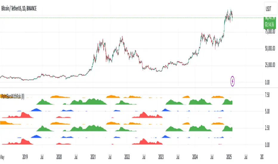
Pragmatic risk managementINTRO
The indicator is calculating multiple moving averages on the value of price change %. It then combines the normalized (via arctan function) values into a single normalized value (via simple average).
The total error from the center of gravity and the angle in which the error is accumulating represented by 4 waves:
BLUE = Good for chance for price to go up
GREEN = Good chance for price to continue going up
ORANGE = Good chance for price to go down
RED = Good chance for price to continue going down
A full cycle of ORANGE\RED\BLUE\GREEN colors will ideally lead to the exact same cycle, if not, try to understand why.
NOTICE-
This indicator is calculating large time-windows so It can be heavy on your device. Tested on PC browser only.
My visual setup:
1. Add two indicators on-top of each other and merge their scales (It will help out later).
2. Zoom out price chart to see the maximum possible data.
3. Set different colors for both indicators for simple visual seperation.
4. Choose 2 different values, one as high as possible and one as low as possible.
(Possible - the indicator remains effective at distinguishing the cycle).
Manual calibration:
0. Select a fixed chart resolution (2H resolution minimum recommended).
1. Change the "mul2" parameter in ranges between 4-15 .
2. Observe the "Turning points" of price movement. (Typically when RED\GREEN are about to switch.)
2. Perform a segmentation of time slices and find cycles. No need to be exact!
3. Draw a square on price movement at place and color as the dominant wave currently inside the indicator.
This procedure should lead to a full price segmentation with easier anchoring.
[blackcat] L2 Ehlers Autocorrelation PeriodogramLevel: 2
Background
John F. Ehlers introduced Autocorrelation Periodogram in his "Cycle Analytics for Traders" chapter 8 on 2013.
Function
Construction of the autocorrelation periodogram starts with the autocorrelation function using the minimum three bars of averaging. The cyclic information is extracted using a discrete Fourier transform (DFT) of the autocorrelation results. This approach has at least four distinct advantages over other spectral estimation techniques. These are:
1. Rapid response. The spectral estimates start to form within a half-cycle period of their initiation.
2. Relative cyclic power as a function of time is estimated. The autocorrelation at all cycle periods can be low if there are no cycles present, for example, during a trend. Previous works treated the maximum cycle amplitude at each time bar equally.
3. The autocorrelation is constrained to be between minus one and plus one regardless of the period of the measured cycle period. This obviates the need to compensate for Spectral Dilation of the cycle amplitude as a function of the cycle period.
4. The resolution of the cyclic measurement is inherently high and is independent of any windowing function of the price data.
The dominant cycle is extracted from the spectral estimate in the next block of code using a center-of-gravity (CG) algorithm. The CG algorithm measures the average center of two-dimensional objects. The algorithm computes the average period at which the powers are centered. That is the dominant cycle. The dominant cycle is a value that varies with time. The spectrum values vary between 0 and 1 after being normalized. These values are converted to colors. When the spectrum is greater than 0.5, the colors combine red and yellow, with yellow being the result when spectrum = 1 and red being the result when the spectrum = 0.5. When the spectrum is less than 0.5, the red saturation is decreased, with the result the color is black when spectrum = 0.
Key Signal
DominantCycle --> Dominant Cycle
Period --> Autocorrelation Periodogram Array
Pros and Cons
100% John F. Ehlers definition translation of original work, even variable names are the same. This help readers who would like to use pine to read his book. If you had read his works, then you will be quite familiar with my code style.
Remarks
The 49th script for Blackcat1402 John F. Ehlers Week publication.
Courtesy of @RicardoSantos for RGB functions.
Readme
In real life, I am a prolific inventor. I have successfully applied for more than 60 international and regional patents in the past 12 years. But in the past two years or so, I have tried to transfer my creativity to the development of trading strategies. Tradingview is the ideal platform for me. I am selecting and contributing some of the hundreds of scripts to publish in Tradingview community. Welcome everyone to interact with me to discuss these interesting pine scripts.
The scripts posted are categorized into 5 levels according to my efforts or manhours put into these works.
Level 1 : interesting script snippets or distinctive improvement from classic indicators or strategy. Level 1 scripts can usually appear in more complex indicators as a function module or element.
Level 2 : composite indicator/strategy. By selecting or combining several independent or dependent functions or sub indicators in proper way, the composite script exhibits a resonance phenomenon which can filter out noise or fake trading signal to enhance trading confidence level.
Level 3 : comprehensive indicator/strategy. They are simple trading systems based on my strategies. They are commonly containing several or all of entry signal, close signal, stop loss, take profit, re-entry, risk management, and position sizing techniques. Even some interesting fundamental and mass psychological aspects are incorporated.
Level 4 : script snippets or functions that do not disclose source code. Interesting element that can reveal market laws and work as raw material for indicators and strategies. If you find Level 1~2 scripts are helpful, Level 4 is a private version that took me far more efforts to develop.
Level 5 : indicator/strategy that do not disclose source code. private version of Level 3 script with my accumulated script processing skills or a large number of custom functions. I had a private function library built in past two years. Level 5 scripts use many of them to achieve private trading strategy.

predict lagUse the angle of multiple moving time windows to calculate the angular momentum vector across time. represent in a spectrum of frequencies\colors\transparency together with the accumulative "truth" (black)

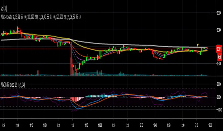
MACD + RSI togetheryou will have both MACD and RSI together in front of each other. best for tile windows or small monitors. enjoy
Better Bollinger Bands (now open source)General purpose Bollinger band indicator with a number of configuration options and some additional color-coded information. The main advantages of it over standard Bollinger bands are:
1) Better statistics:
* Uses volume weighted moving averages, variance, and standard deviation by default. The volume dependence can be disabled with a checkbox option, but generally makes it more responsive improves its ability to distinguish true outlier events from random variation.
* Lets you pick between different time windows (simple, sawtooth (WMA), exponential) in addition to the volume weighting, with appropriate Bessel corrections to make the estimators unbiased and to get consistent result for different weights.
* Has a checkbox option to use a linear regression in the band calculation if you don't want average momentum to be counted in the volatility. This turns the centerline into a last squares moving average, and the band width at each time step is given by the variance away from the regression line instead of from a moving average. Weights in the least squares regression are changed according to the other options. For tickers with a strong long-term trend this makes the bands track the price action more closely.
2) Geometric
* This does all calculations on log(price) instead of the prices themselves.
* Makes almost no difference in most cases, but gives better results on charts with strongly exponential behaviour that range between several orders of magnitude.
* Properly centered around price action on log plots.
* Will never annoy you by rescaling a log plot due to a negative lower band. The lower band is always positive for positive prices.
3) Some built in oscillators.
* This aims to reduce clutter by building in some other indicators into the band color scheme. You can pick between various momentum & RSI operators to color the center line and the bands, or leave the bands plain.
I've been using these bands myself for a few months & have been gradually adding functionality & polish. Feel free to comment, or to refer to me if you borrow any ideas.

FREE TRADINGVIEW FOR TIMEFRAMESWhen doing i.e the 3 minute timeframe turn on the closest timeframe available for you or the candles and wicks will be fucked up.
So if you're doing the 5 hour timeframe candles turn on the 4hr chart on your main chart.
To View the candles in full screen double click the windows with the candlesticks
If you don't have TradingView premium and want to look at custom timeframes you can use this.
For the ticker/coin/pair you want to show enter it like this:
For stocks, only the ticker i.e: MSFT, APPL
For Crypto, "Exchange:ticker" i.e: BITFINEX:BTCUSD, BINANCE:AGIBTC, BITMEX:ADAM19
When setting up the timeframe write i.e:
For minutes/hourly: 5, 240 (4 hour), 360 (6 hour)
For daily/weekly/monthly: 1D, 2W, 3M
When doing i.e the 3 minute timeframe turn on the closest timeframe available for you or the candles and wicks will be fucked up.
So if you're doing the 5 hour timeframe candles turn on the 4hr chart on your main chart.

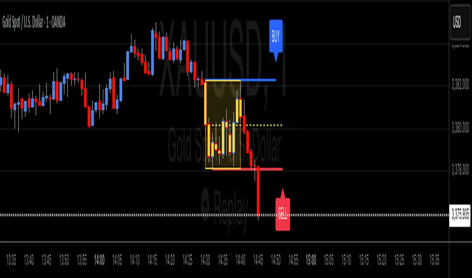
ORB Breakouts with alerts"ORB Breakouts with Alerts" is a utility indicator that highlights an Opening Range Breakout (ORB) setup during a user-defined intraday time window. It allows traders to visualize price consolidation ranges and receive alerts when price breaks above or below the session high/low.
🔧 Features:
*Customizable session time (start and end), adjustable to local time using a timezone offset.
*Automatically plots:
*A shaded box around the session's high and low.
*Horizontal lines at session high and low levels.
*Optional "BUY"/"SELL" labels to mark breakout directions.
*Visual breakout signals when price crosses above or below the session range.
*Built-in alerts to notify when breakouts occur.
*Configurable styling options including box color, highlight color, and label placement.
⚙️ How It Works:
*During the defined time range, the script tracks the highest high and lowest low.
*After the session ends:
*A box is drawn to represent the opening range.
*Breakouts above the high or below the low trigger visual markers and optional alerts.
*Alerts are limited to one per direction per day to reduce noise.
⚠️ This indicator is a technical analysis tool only and does not provide financial advice or trade recommendations. Always use with proper risk management and in conjunction with your trading plan.
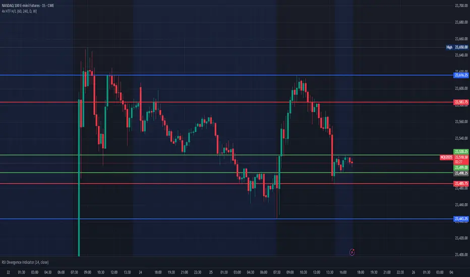
Multi HTF High/Low LevelsThis indicator plots the previous high and low from up to four user-defined higher timeframes (HTF), providing crucial levels of support and resistance. It's designed to be both powerful and clean, giving you a clear view of the market structure from multiple perspectives without cluttering your chart.
Key Features:
Four Customizable Timeframes: Configure up to four distinct higher timeframes (e.g., 1-hour, 4-hour, Daily, Weekly) to see the levels that matter most to your trading style.
Automatic Visibility: The indicator is smart. It automatically hides levels from any timeframe that is lower than your current chart's timeframe. For example, if you're viewing a Daily chart, the 4-hour levels won't be shown.
Clean On-Chart Lines: The high and low for each timeframe are displayed as clean, extended horizontal lines, but only for the duration of the current higher-timeframe period. This keeps your historical chart clean while still showing the most relevant current levels.
Persistent Price Scale Labels: For easy reference, the price of each high and low is always visible on the price scale and in the data window. This is achieved with an invisible plot, giving you the accessibility of a plot without the visual noise.
How to Use:
Go into the indicator settings.
Under each "Timeframe" group, check the "Show" box to enable that specific timeframe.
Select your desired timeframe from the dropdown menu.
The indicator will automatically calculate and display the previous high and low for each enabled timeframe.
Trade Calculator {Phanchai}Trade Calculator 🧮 {Phanchai} — Documentation
A lightweight sizing helper for TradingView that turns your risk per trade into an estimated maximum nominal position size — using the most recent chart low as your stop reference. Built for speed and clarity right on the chart.
Key Features
Clean on-chart info table with configurable font size and position.
Row toggles: show/hide each line (Price, Last Low, Risk per Trade, Entry − Low, SL to Low %, Max. Nominal Value in USDT).
Configurable low reference: Last N bars or Running since load .
Low label placed exactly at the wick of the lowest bar (no horizontal line).
Custom padding: add extra rows above/below and blank columns left/right (with custom whitespace/text fillers) to fine-tune layout.
Integer display for Risk per Trade (USDT) and Max. Nominal Value (USDT); decimals configurable elsewhere.
Open source script — easy to read and extend.
How to Use
Add the indicator: open TradingView → Indicators → paste the source code → Add to chart.
Pick your low reference in settings:
Last N bars — uses the lowest low within your chosen lookback.
Running since load — tracks the lowest low since the script loaded.
Set your capital and risk:
Total Capital — your account size in USDT.
Max. invest Capital per Trade (%) — your risk per trade as a percent of Total Capital.
Tidy the table:
Use Table Position and Table Size to place it.
Add Extra rows/columns and set left/right fillers (spaces allowed) for padding.
Toggle individual rows (on/off) to show only what you need.
Read the numbers:
Act. Price in USDT — current close.
Last Low in USDT — stop reference price.
Risk per Trade — whole-USDT value of your risk budget for this trade.
Entry − Low — absolute risk per unit.
SL to Low (%) — percentage distance from price to low.
Max. Nominal Value in USDT — estimated max nominal position size given your risk budget and stop at the low.
Scope
This calculator is designed for long trades only (stop below price at the chart low).
Notes & Assumptions
Does not factor fees, funding, slippage, tick size, or broker/venue position limits.
“Running since load” updates as new lows appear; “Last N bars” uses only the selected lookback window.
If price equals the low (zero distance), sizing will be undefined (division by zero guarded as “—”).
Risk Warning
Trading involves substantial risk. Always double-check every value the calculator shows, confirm your stop distance, and verify position sizing with your broker/platform before entering any order. Never risk money you cannot afford to lose.
Open Source & Feedback
The source code is open. If you spot a bug or have an idea to improve the tool, feel free to share suggestions — I’m happy to iterate and make it better.

Custom ORBIT — GSK-VIZAG-AP-INDIA 📌 Description
Custom ORBIT — Opening Range Breakout Indicator Tool
Created by GSK-VIZAG-AP-INDIA
This indicator calculates and visualizes the Opening Range (OR) of the trading session, with customizable start/end times and flexible range duration. The Opening Range is defined by the highest and lowest prices during the selected initial market window.
🔹 Key Features:
User-defined Opening Range duration (default: 15 minutes from 9:15).
Adjustable session start and end times.
Plots Opening Range High (ORH) and Opening Range Low (ORL).
Extends OR levels across the session with multiple line style options (Dotted, Dashed, Solid, Smoothed).
Highlights breakouts (price crossing above/below OR) and reversals (price returning back inside).
Simple chart markers (triangles/labels) for quick visual recognition.
⚠️ Disclaimer:
This tool is intended for educational and analytical purposes only. It does not generate buy/sell signals or provide financial advice. Always use independent analysis and risk management.

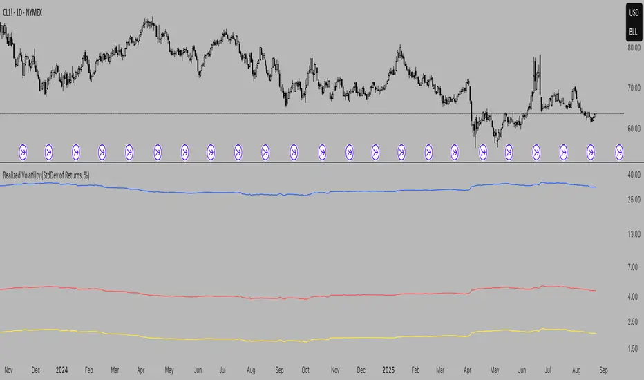
Realized Volatility (StdDev of Returns, %)Realized Volatility (StdDev of Returns, %)
This indicator measures realized (historical) volatility by calculating the standard deviation of log returns over a user-defined lookback period. It helps traders and analysts observe how much the price has varied in the past, expressed as a percentage.
How it works:
Computes close-to-close logarithmic returns.
Calculates the standard deviation of these returns over the selected lookback window.
Provides three volatility measures:
Daily Volatility (%): Standard deviation over the chosen period.
Annualized Volatility (%): Scaled using the square root of the number of trading days per year (default = 250).
Horizon Volatility (%): Scaled to a custom horizon (default = 5 days, useful for short-term views).
Inputs:
Lookback Period: Number of bars used for volatility calculation.
Trading Days per Year: Used for annualizing volatility.
Horizon (days): Adjusts volatility to a shorter or longer time frame.
Notes:
This is a statistical measure of past volatility, not a forecasting tool.
If you change the scale to logarithmic, the indicator readibility improves.
It should be used for analysis in combination with other tools and not as a standalone signal.
On-Balance Volume with Multiple MA TypesOn-Balance Volume with Multiple MA Types
English Description
Overview
This is the first version of the "On-Balance Volume with Multiple MA Types" indicator designed to overlay directly on the price chart, a significant evolution from its previous iterations, which functioned solely as an oscillator in a separate window. The indicator calculates On-Balance Volume (OBV) and applies various smoothing methods to provide a clear view of volume dynamics in relation to price movements. It is pinned to the price scale for seamless integration with the chart.
Interpretation Recommendations
Price Pushing the OBV Line from Below: When the price chart pushes the OBV line upward and remains below it, this indicates rising volume, suggesting strong buying pressure.
Price Above the OBV Line: When the price chart is above the OBV line, it signals falling volume, indicating weakening momentum or selling pressure.
OBV Line Crossings: When the price crosses the OBV line, it represents a balance point in volume dynamics. The price level at the current crossing can be compared to the previous crossing to assess changes in market sentiment or momentum.
Moving Average Types
The indicator offers eight smoothing options for the OBV line, each with unique characteristics:
EMA (Exponential Moving Average): A weighted average that prioritizes recent data, providing a smooth yet responsive line.
DEMA (Double Exponential Moving Average): Uses two EMAs to reduce lag, offering faster response to volume changes.
HMA (Hull Moving Average): Combines weighted moving averages to minimize lag while maintaining smoothness.
WMA (Weighted Moving Average): Assigns more weight to recent data, balancing responsiveness and noise reduction.
TMA (Triangular Moving Average): A double-smoothed simple moving average, emphasizing central data points for smoother output.
VIDYA (Variable Index Dynamic Average): Adapts smoothing based on market volatility, using a CMO (Chande Momentum Oscillator) for dynamic weighting. Controlled by the VIDYA Alpha parameter (default: 0.2, range: 0–1), which adjusts sensitivity to volatility.
FRAMA (Fractal Adaptive Moving Average): Adjusts smoothing based on fractal dimensions of the OBV data, adapting to market conditions.
JMA (Jurik Moving Average): A proprietary adaptive average designed for minimal lag and high smoothness. Controlled by two parameters:
JMA Phase (default: 50, range: -100 to 100): Adjusts the balance between responsiveness and smoothness.
JMA Power (default: 1, range: 0.1+): Controls the strength of smoothing.
Input Parameters
OBV MA Length (default: 10): The lookback period for smoothing the OBV. Higher values produce smoother results but increase lag.
OBV MA Type (default: JMA): Selects the moving average type from the eight options listed above.
Line Width (default: 2): Thickness of the OBV line on the chart.
Bullish Color (default: Blue): Color of the OBV line when rising (indicating increasing volume).
Bearish Color (default: Red): Color of the OBV line when falling (indicating decreasing volume).
JMA Phase (default: 50): Adjusts the JMA’s responsiveness (used only when JMA is selected).
JMA Power (default: 1): Adjusts the JMA’s smoothing strength (used only when JMA is selected).
VIDYA Alpha (default: 0.2): Controls the sensitivity of VIDYA to market volatility (used only when VIDYA is selected).
How to Use
Add the indicator to your TradingView chart. It will overlay directly on the price chart, aligned with the price scale.
Adjust the OBV MA Type to select your preferred smoothing method based on your trading style (e.g., JMA for low lag, TMA for smoothness).
Modify the OBV MA Length to balance responsiveness and noise reduction. Shorter periods (e.g., 5–10) are better for short-term trading, while longer periods (e.g., 20–50) suit longer-term analysis.
Use the Bullish Color and Bearish Color to visually distinguish rising and falling volume trends.
For JMA or VIDYA, fine-tune the JMA Phase, JMA Power, or VIDYA Alpha to optimize the indicator for specific market conditions.
Interpret the OBV line in relation to price:
Watch for price pushing the OBV line upward (rising volume) or moving above it (falling volume).
Note crossings of the OBV line to identify balance points and compare with prior crossings to gauge momentum shifts.
Combine with other technical tools (e.g., support/resistance levels, trendlines) for a comprehensive trading strategy.
Notes
This indicator is designed to work on any timeframe and market, but its effectiveness depends on the chosen moving average type and parameters.
Experiment with different MA types and lengths to find the best fit for your trading approach.
The indicator is licensed under the Mozilla Public License 2.0 and copyrighted by TradingStrategyCourses © 2025.

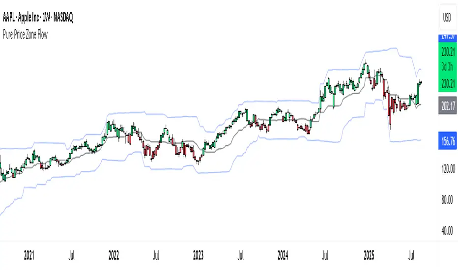
Pure Price Zone Flow🔎 What this indicator is
It’s a price-action-based zone indicator. Unlike moving average systems, this one relies only on:
1. Swing Highs & Swing Lows → The highest and lowest points within a recent lookback period (like "mini support & resistance").
2. ATR (Average True Range) → A volatility measure that expands the zone, making it more adaptive to different market conditions.
3. Breakouts & Retests → When price breaks above a swing high (bullish) or below a swing low (bearish), the indicator marks it and highlights the new trend.
👉 The goal is to spot clean structure shifts and define clear trend zones where traders can position themselves.
________________________________________
⚙️ How it is calculated
1. Swing High & Swing Low
o We look back len candles (default 20).
o Find the highest high (swingHigh) and the lowest low (swingLow) in that window.
o This forms the price range zone.
2. ATR Expansion
o We calculate ATR over the same len.
o Add/subtract it (multiplied by atrMult) to the zone edges to expand them.
o This ensures the zones breathe with volatility (tight in quiet markets, wide in choppy ones).
3. Mid-Zone
o Simply the average of swingHigh and swingLow.
o If price is above mid → bullish bias.
o If below mid → bearish bias.
o This gives us the trend color for candles.
4. Breakouts
o If the close crosses above swingHigh, we mark a bullish breakout with a label.
o If the close crosses below swingLow, we mark a bearish breakdown.
________________________________________
📊 How it helps traders
This indicator helps by:
1. Identifying Structure Shifts
o Many traders watch swing highs/lows for breakouts or reversals.
o This automates the process and visually confirms when structure is broken.
2. Dynamic Zone Trading
o Instead of fixed support/resistance, the ATR expansion adapts to volatility.
o This avoids false signals in high-volatility conditions.
3. Trend Bias at a Glance
o Candle coloring instantly tells you whether price is in bullish or bearish territory relative to the mid-zone.
4. Breakout Confirmation
o The labels show when a breakout has occurred, so traders can react quickly (e.g., enter with trend, wait for retest, or avoid fading moves).
________________________________________
🌍 Markets it works best in
• Crypto (Bitcoin, Ethereum, etc.): Very effective since crypto is breakout-driven and respects swing levels.
• Forex: Good for volatility-adaptive structure analysis, especially in trending pairs.
• Indices (SPX, NASDAQ, DAX, NIFTY): Useful for breakout trading during session opens or key news events.
• Commodities (Gold, Oil, Silver): Works well to define intraday ranges and breakout levels.
⚠️ Less useful in low-volatility, mean-reverting assets (like some penny stocks or sideways ranges), because breakouts may be rare or fake.
________________________________________
💡 How it adds value
• Strips away unnecessary complexity (no lagging averages).
• Focuses directly on what price is doing structurally.
• Adaptive → works across different markets & timeframes.
• Easy visualization → zones, trend coloring, breakout markers.
• Helps traders trade with the flow of the market, instead of guessing tops/bottoms.
________________________________________
👉 In short:
This indicator turns raw price action into clear, actionable zones.
It highlights when the market shifts from balance to breakout, so traders can align with momentum rather than fighting it.
FlowScape PredictorFlowScape Predictor is a non-repainting, regime-aware entry qualifier that turns complex market context into two readiness scores (Long & Short, each 0/25/50/75/100) and clean, confirmed-bar signals. It blends three orthogonal pillars so you act only when trend energy, momentum, and location agree:
Regime (energy): ATR-normalized linear-regression slope of a smooth HMA → EMA baseline, gated by ADX to confirm when pressure is meaningful.
Momentum (push): RSI slope alignment so price has directional follow-through, not just drift.
Structure (location): proximity to pivot-confirmed swings, scaled by ATR, so “ready” appears near constructive pullbacks—not mid-trend chases.
A soft ATR cloud wraps the baseline for context. A yellow Predictive Baseline extends beyond the last bar to visualize near-term trajectory. It is visual-only: scores/alerts never use it.
What you see
Baseline line that turns green/red when regime is strong in that direction; gray when weak.
ATR cloud around the baseline (context for stretch and pullbacks).
Scores (Long & Short, 0–100 in steps of 25) and optional “L/S” icons on bar close.
Yellow Predictive Baseline that extends to the right for a few bars (visual trajectory of the smoothed baseline).
The scoring system (simple and transparent)
Each side (Long/Short) sums four binary checks, 25 points each:
Regime aligned: trendStrong is true and LR slope sign favors that side.
Momentum aligned: RSI side (>50 for Long, <50 for Short) and RSI slope confirms direction.
Baseline side: price is above (Long) / below (Short) the baseline.
Location constructive: distance from the last confirmed pivot is healthy (ATR-scaled; not overstretched).
Valid totals are 0, 25, 50, 75, 100.
Best-quality signal: 100/0 (your side/opposite) on bar close.
Good, still valid: 75/0, especially when the missing block is only “location” right as price re-engages the cloud/baseline.
Avoid: 75/25 or any opposition > 0 in a weak (gray) regime.
The Predictive (Kalman) line — what it is and isn’t
The yellow line is a visual forward extension of the smoothed baseline to help you see the current trajectory and time pullback resumptions. It does not predict price and is excluded from scores and alerts.
How it’s built (plain English):
We maintain a one-dimensional Kalman state x as a smoothed estimate of the baseline. Each bar we observe the current baseline z.
The filter adjusts its trust using the Kalman gain K = P / (P + R) and updates:
x := x + K*(z − x), then P := (1 − K)*P + Q.
Q (process noise): Higher Q → expects faster change → tracks turns quicker (less smoothing).
R (measurement noise): Higher R → trusts raw baseline less → smoother, steadier projection.
What you control:
Lead (how many bars forward to draw).
Kalman Q/R (visual smoothness vs. responsiveness).
Toggle the line on/off if you prefer a minimal chart.
Important: The predictive line extends the baseline, not price. It’s a visual timing aid—don’t automate off it.
How to use (step-by-step)
Keep the chart clean and use a standard OHLC/candlestick chart.
Read the regime: Prefer trades with green/red baseline (trendStrong = true).
Check scores on bar close:
Take Long 100 / Short 0 or Long 75 / Short 0 when the chart shows a tidy pullback re-engaging the cloud/baseline.
Mirror the logic for shorts.
Confirm location: If price is > ~1.5 ATR from its reference pivot, let it come back—avoid chasing.
Set alerts: Add an alert on Long Ready or Short Ready; these fire on closed bars only.
Risk management: Use ATR-buffered stops beyond the recent pivot; target fixed-R multiples (e.g., 1.5–3.0R). Manage the trade with the baseline/cloud if you trail.
Best-practice playbook (quick rules)
Green light: 100/0 (best) or 75/0 (good) on bar close in a colored (non-gray) regime.
Location first: Prefer entries near the baseline/cloud right after a pullback, not far above/below it.
Avoid mixed signals: Skip 75/25 and anything with opposition while the baseline is gray.
Use the yellow line with discretion: It helps you see rhythm; it’s not a signal source.
Timeframes & tuning (practical defaults)
Intraday indices/FX (5m–15m): Demand 100/0 in chop; allow 75/0 when ADX is awake and pullback is clean.
Crypto intraday (15m–1h): Prefer 100/0; 75/0 on the first pullback after a regime turn.
Swing (1h–4h/D1): 75/0 is often sufficient; 100/0 is excellent (fewer but cleaner signals).
If choppy: raise ADX threshold, raise the readiness bar (insist on 100/0), or lengthen the RSI slope window.
What makes FlowScape different
Energy-first regime filter: ATR-normalized LR slope + ADX gate yields a consistent read of trend quality across symbols and timeframes.
Location-aware entries: ATR-scaled pivot proximity discourages mid-air chases, encouraging pullback timing.
Separation of concerns: The predictive line is visual-only, while scores/alerts are confirmed on close for non-repainting behavior.
One simple score per side: A single 0–100 readiness figure is easier to tune than juggling multiple indicators.
Transparency & limitations
Scores are coarse by design (25-point blocks). They’re a gatekeeper, not a promise of outcomes.
Pivots confirm after right-side bars, so structure signals appear after swings form (non-repainting by design).
Avoid using non-standard chart types (Heikin Ashi, Renko, Range, etc.) for signals; use a clean, standard chart.
No lookahead, no higher-timeframe requests; alerts fire on closed bars only.

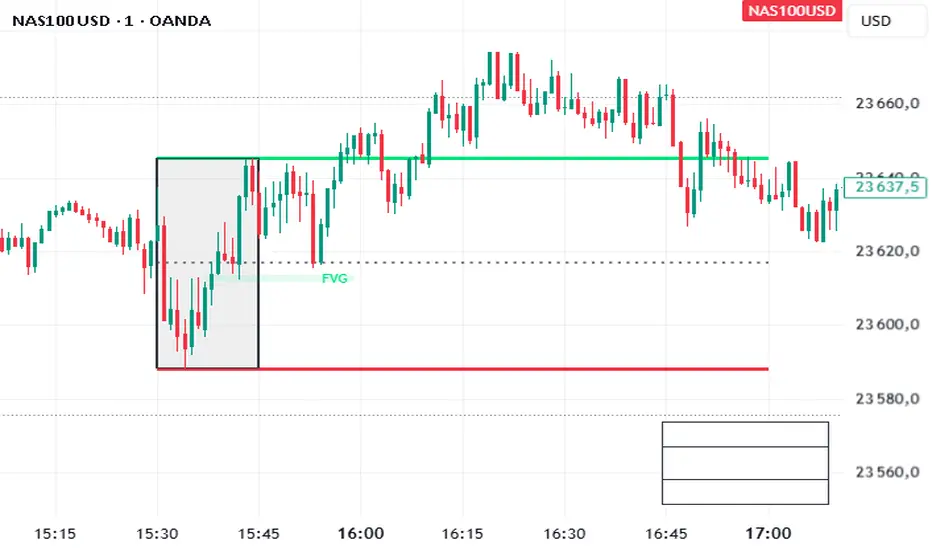
OPR — DAX or USEnglish
This indicator automatically plots the Opening Price Range (OPR) for different indices, with customizable start and end times for each instrument.
For the DAX, it draws the high (green), low (red), and midline (grey dotted) for the specified range, defaulting to 09:00–09:15, and extends the lines until the selected end time (default 11:00).
For US indices (Dow Jones, Nasdaq, S&P500), it applies the same logic for the default 15:30–15:45 range, with two vertical black bars marking the start and end of the time window.
Each symbol only displays its own relevant lines (e.g., viewing DAX will only show DAX markers).
Parameters allow adjusting times and visibility for each market.
Entropy (Fiedor/Kontoyiannis) - Part 2 of Fiedor's TheoryThis indicator estimates the Shannon entropy of a price series using a Markov chain model of binary returns, following the approach of Fiedor (2014) and Kontoyiannis (1997).
% of Max shows current entropy as a percentage of its theoretical maximum (1 bit for binary up/down moves).
Percentile ranks the current entropy against historical values in the chosen lookback window.
High entropy suggests price movement is less predictable by frequentist models; low entropy implies more structure and predictability.
Use this as an informational oscillator, not a trading signal.
This is a visualization of Part 1 of Fiedor's Theory. The same entropy logic is already embedded in Part 1 however the second pane is a nice reminder of why it works.

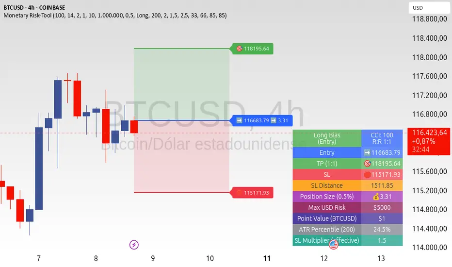
ATR+CCI Monetary Risk Tool - TP/SL⚙️ ATR+CCI Monetary Risk Tool — Volatility-aware TP/SL & Position Sizing
Exact prices (no rounding), ATR-percentile dynamic stops, and risk-budget sizing for consistent execution.
🧠 What this indicator is
A risk-first planning tool. It doesn’t generate orders; it gives you clean, objective levels (Entry, SL, TP) and position size derived from your risk budget. It shows only the latest setup to keep charts readable, and a compact on-chart table summarizing the numbers you actually act on.
✨ What makes it different
Dynamic SL by regime (ATR percentile): Instead of a fixed multiple, the SL multiplier adapts to the current volatility percentile (low / medium / high). That helps avoid tight stops in noisy markets and over-wide stops in quiet markets.
Risk budgeting, not guesswork: Size is computed from Account Balance × Max Risk % divided by SL distance × point value. You risk the same dollars across assets/timeframes.
Precision that matches your instrument: Entry, TP, SL, and SL Distance are displayed as exact prices (no rounding), truncated to syminfo.mintick so they align with broker/exchange precision.
Symbol-aware point value: Uses syminfo.pointvalue so you don’t maintain tick tables.
Non-repaint option: Work from closed bars to keep the plan stable.
🔧 How to use (quick start)
Add to chart and pick your timeframe and symbol.
In settings:
Set Account Balance (USD) and Max Risk per Trade (%).
Choose R:R (1:1 … 1:5).
Pick ATR Period and CCI Period (defaults are sensible).
Keep Dynamic ATR ON to adapt SL by regime.
Keep Use closed-bar values ON to avoid repaint when planning.
Read the labels (Entry/TP/SL) and the table (SL Distance, Position Size, Max USD Risk, ATR Percentile, effective SL Mult).
Combine with your entry trigger (price action, levels, momentum, etc.). This indicator handles risk & targets.
📐 How levels are computed
Bias: CCI ≥ 0 ⇒ long, otherwise short.
ATR Percentile: Percent rank of ATR(atrPeriod) over a lookback window.
Effective SL Mult:
If percentile < Low threshold ⇒ use Low SL Mult (tighter).
If between thresholds ⇒ use Base SL Mult.
If percentile > High threshold ⇒ use High SL Mult (wider).
Stop-Loss: SL = Entry ± ATR × SL_Mult (minus for long, plus for short).
Take-Profit: TP = Entry ± (Entry − SL) × R (R from the R:R dropdown).
Position Size:
USD Risk = Balance × Risk%
Contracts = USD Risk ÷ (|Entry − SL| × PointValue)
For futures, quantity is floored to whole contracts.
Exact prices: Entry/TP/SL and SL Distance are not rounded; they’re truncated to mintick so what you see matches valid price increments.
📊 What you’ll see on chart
Latest Entry (blue), TP (green), SL (red) with labels (optional emojis: ➡️ 🎯 🛑).
Info Table with:
Bias, Entry, TP, SL (exact, truncated to mintick)
SL Distance (exact, truncated)
Position Size (contracts/units)
Max USD Risk
Point Value
ATR Percentile and effective SL Mult
🧪 Practical examples
High-volatility session (e.g., XAUUSD, 1H): ATR percentile is high ⇒ wider SL, smaller size. Reduces churn from normal noise during macro events.
Range-bound market (e.g., EURUSD, 4H): ATR percentile low ⇒ tighter SL, better R:R. Helps you avoid carrying unnecessary risk.
Index swing planning (e.g., ES1!, Daily): Non-repaint levels + risk budgeting = consistent sizing across days/weeks, easier to review and journal.
🧭 Why traders should use it
Consistency: Same dollar risk regardless of instrument or volatility regime.
Clarity: One-trade view forces focus; you see the numbers that matter.
Adaptivity: Stops calibrated to the market’s current behavior, not last month’s.
Discipline: A visible checklist (SL distance, size, USD risk) before you hit buy/sell.
🔧 Input guide (practical defaults)
CCI Period: 100 by default; use as a bias filter, not an entry signal.
ATR Period: 14 by default; raise for smoother, lower for more reactive.
ATR Percentile Lookback: 200 by default (stable regime detection).
Percentile thresholds: 33/66 by default; widen the gap to change how often regimes switch.
SL Mults: Start ~1.5 / 2.0 / 2.5 (low/base/high). Tune by asset.
Risk % per trade: Common pro ranges are 0.25–1.0%; adjust to your risk tolerance.
R:R: Start with 1:2 or 1:3 for balanced skew; adapt to strategy edge.
Closed-bar values: Keep ON for planning/live; turn OFF only for exploration.
💡 Best practices
Combine with your entry logic (structure, momentum, liquidity levels).
Review ATR percentile and effective SL Mult across sessions so you understand regime shifts.
For futures, remember size is floored to whole contracts—safer by design.
Journal trades with the table snapshot to improve risk discipline over time.
⚠️ Notes & limitations
This is not a strategy; it does not place orders or alerts.
No slippage/commissions modeled here; build a strategy() version for backtests that mirror your broker/exchange.
Displayed non-price metrics use two decimals; prices and SL Distance are exact (truncated to mintick).
📎 Disclaimer
For educational purposes only. Not financial advice. Markets involve risk. Test thoroughly before trading live.
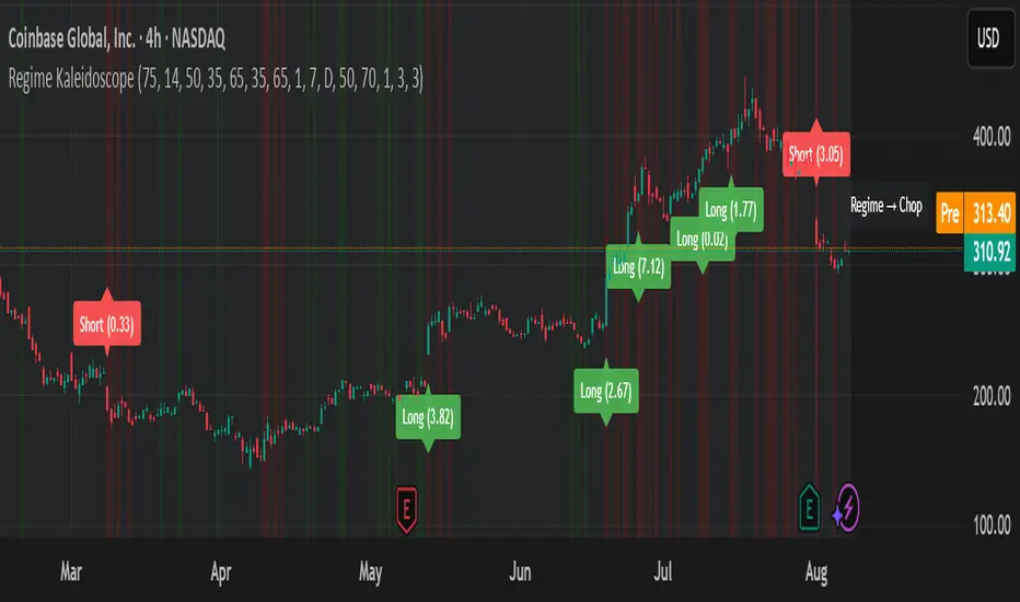
Regime KaleidoscopeWhat is Regime Kaleidoscope?
Regime Kaleidoscope is an advanced market regime visualizer and adaptive signal generator.
It helps traders instantly understand whether current market conditions are best for mean-reversion (fading price back to the mean) or breakout/trend-following (riding strong moves), using a data-driven, non-repainting approach.
How It Works
1. Regime Detection & Background Colors
The indicator analyzes both volatility (ATR) and the shape of each candle (body size vs. range) over a rolling window.
Each bar is classified into one of three regimes, and the chart’s background color changes accordingly:
Regime Background Color What It Means How to Use
Low Vol Balanced Green background Market is calm, compressed. More likely to revert back to mean. Look for mean-reversion signals only (fade moves).
High Vol Directional Red background Market is in a high-volatility, trending, or “breakout” state.
Red does NOT mean bearish. It simply means conditions are ripe for strong directional moves—either up or down. Look for breakout signals only (ride strong moves after structure break).
Chop Gray background Market is indecisive or transitioning between states. Signals are minimized or blocked. Best to wait or trade with extra caution.
→ Red background means high volatility/trending regime, not a signal direction!
Green means “mean-revert environment,” not always bullish!
Gray means “chop/transition”—usually best avoided.
2. Signals — How to Read and Trade Them
Mean-Reversion Signals (Green Regime Only):
Appear when price is stretched away from a rolling mean (SMA) by a configurable ATR-based threshold.
Optional: Only allowed in the direction of the higher-timeframe trend, if enabled.
Long signals: Fade extreme dips (look for triangle-up shapes & green labels).
Short signals: Fade extreme spikes (triangle-down shapes & red labels).
Labels show signal strength (distance from mean in ATR units).
Breakout Signals (Red Regime Only):
Only triggered when price breaks above or below a confirmed swing high or low (pivot), with a strong candle and optional trend confirmation.
Long signals: Breakout above last swing high (regardless of background color).
Short signals: Breakout below last swing low.
Labels show signal strength (distance from pivot in ATR units).
Red background does NOT mean sell— it means “trend environment”—so both long and short signals are possible, depending on which direction price is breaking out.
Signal Controls & Filtering:
Signals only fire at bar close (non-repainting), never intrabar or on future data.
ATR “floor” blocks signals when volatility is too low for meaningful moves.
Cooldown: Signals are limited to one per regime per direction for a minimum number of bars (user input).
Optional confirmation candles: Only strong reversals or breakouts count, reducing noise and whipsaws.
All signals are visible as triangle shapes below/above bars, and labeled with strength.
3. Visual Guide
Background color: Maps the regime, not buy/sell direction.
Transition label: Appears only when the regime changes, so you can see state shifts at a glance.
Triangle shapes & labels: Mark entry points; label gives strength.
Info table (optional): Shows regime and ATR at transitions.
Why is Regime Kaleidoscope Unique?
Uses rolling statistical percentiles of ATR and candle body shape for dynamic market state detection—not just a moving average or volatility band.
Separates regime from signal direction, so you always know “what mode the market is in” and when signals actually have a higher probability.
No repainting. All logic is strictly bar-close, confirmed pivots, and non-future-leaking.
Highly customizable—all thresholds, filters, trend confirmation, and cooldown are user inputs.
How To Use
Add to any chart.
Use the background color to identify if you’re in a mean-revert, breakout, or chop regime.
Take only the signals that match the regime:
Green = fade extremes, Red = ride breakouts, Gray = wait.
Tune settings for your asset and timeframe.
All signals are educational—always test before live use!
Past performance is not necessarily indicative of future results.
Test the indicator on your assets and timeframes. All signals are for educational use only.
thors_forex_factory_utilityLibrary "forex_factory_utility"
Supporting Utility Library for the Live Economic Calendar by toodegrees Indicator; responsible for data handling, and plotting news event data.
isLeapYear()
Finds if it's currently a leap year or not.
Returns: Returns True if the current year is a leap year.
daysMonth(M)
Provides the days in a given month of the year, adjusted during leap years.
Parameters:
M (int) : Month in numerical integer format (i.e. Jan=1).
Returns: Days in the provided month.
MMM(M)
Converts a month from a numerical integer format to a MMM format (i.e. 'Jan').
Parameters:
M (int) : Month in numerical integer format (i.e. Jan=1).
Returns: Month in MMM format (i.e. 'Jan').
dow(D)
Converts a numbered day of the week string in format to 'DDD' format (i.e. "1" = Sun).
Parameters:
D (string) : Numbered day of the week from 1 to 7, starting on Sunday.
Returns: Returns the day of the week in 'DDD' format (i.e. "Fri").
size(S, N)
Converts a size string into the corresponding Pine Script v5 format, or N times smaller/bigger.
Parameters:
S (string) : Size string: "Tiny", "Small", "Normal", "Large", or "Huge".
N (int) : Size variation, can be positive (larger than S), or negative (smaller than S).
Returns: Size string in Pine Script v5 format.
lineStyle(S)
Converts a line style string into the corresponding Pine Script v5 format.
Parameters:
S (string) : Line style string: "Dashed", "Dotted" or "Solid".
Returns: Line style string in Pine Script v5 format.
lineTrnsp(S)
Converts a transparency style string into the corresponding integer value.
Parameters:
S (string) : Line style string: "Light", "Medium" or "Heavy".
Returns: Transparency integer.
boxLoc(X, Y)
Converts position strings of X and Y into a table position in Pine Script v5 format.
Parameters:
X (string) : X-axis string: "Left", "Center", or "Right".
Y (string) : Y-axis string: "Top", "Middle", or "Bottom".
Returns: Table location string in Pine Script v5 format.
method bubbleSort_NewsTOD(N)
Performs bubble sort on a Forex Factory News array of all news from the same date, ordering them in ascending order based on the time of the day.
Namespace types: array
Parameters:
N (array) : Forex Factory News array.
Returns: void
bubbleSort_News(N)
Performs bubble sort on a Forex Factory News array, ordering them in ascending order based on the time of the day, and date.
Parameters:
N (array) : Forex Factory News array.
Returns: Sorted Forex Factory News array.
weekNews(N, C, I)
Creates a Forex Factory News array containing the current week's Forex Factory News.
Parameters:
N (array) : Forex Factory News array containing this week's unfiltered Forex Factory News.
C (array) : Currency filter array (string array).
I (array) : Impact filter array (color array).
Returns: Forex Factory News array containing the current week's Forex Factory News.
todayNews(W, D, M)
Creates a Forex Factory News array containing the current day's Forex Factory News.
Parameters:
W (array) : Forex Factory News array containing this week's Forex Factory News.
D (array) : Forex Factory News array for the current day's Forex Factory News.
M (bool) : Boolean that marks whether the current chart has a Day candle-switch at Midnight New York Time.
Returns: Forex Factory News array containing the current day's Forex Factory News.
adjustTimezone(N, TZH, TZM)
Transposes the Time of the Day, and Date, in the Forex Factory News Table to a custom Timezone.
Parameters:
N (array) : Forex Factory News array.
TZH (int) : Custom Timezone hour.
TZM (int) : Custom Timezone minute.
Returns: Reformatted Forex Factory News array.
NewsAMPM_TOD(N)
Reformats the Time of the Day in the Forex Factory News Table to AM/PM format.
Parameters:
N (array) : Forex Factory News array.
Returns: Reformatted Forex Factory News array.
impFilter(X, L, M, H)
Creates a filter array from the User's desired Forex Facory News to be shown based on Impact.
Parameters:
X (bool) : Boolean - if True Holidays listed on Forex Factory will be shown.
L (bool) : Boolean - if True Low Impact listed on Forex Factory News will be shown.
M (bool) : Boolean - if True Medium Impact listed on Forex Factory News will be shown.
H (bool) : Boolean - if True High Impact listed on Forex Factory News will be shown.
Returns: Color array with the colors corresponding to the Forex Factory News to be shown.
curFilter(A, C1, C2, C3, C4, C5, C6, C7, C8, C9)
Creates a filter array from the User's desired Forex Facory News to be shown based on Currency.
Parameters:
A (bool) : Boolean - if True News related to the current Chart's symbol listed on Forex Factory will be shown.
C1 (bool) : Boolean - if True News related to the Australian Dollar listed on Forex Factory will be shown.
C2 (bool) : Boolean - if True News related to the Canadian Dollar listed on Forex Factory will be shown.
C3 (bool) : Boolean - if True News related to the Swiss Franc listed on Forex Factory will be shown.
C4 (bool) : Boolean - if True News related to the Chinese Yuan listed on Forex Factory will be shown.
C5 (bool) : Boolean - if True News related to the Euro listed on Forex Factory will be shown.
C6 (bool) : Boolean - if True News related to the British Pound listed on Forex Factory will be shown.
C7 (bool) : Boolean - if True News related to the Japanese Yen listed on Forex Factory will be shown.
C8 (bool) : Boolean - if True News related to the New Zealand Dollar listed on Forex Factory will be shown.
C9 (bool) : Boolean - if True News related to the US Dollar listed on Forex Factory will be shown.
Returns: String array with the currencies corresponding to the Forex Factory News to be shown.
FF_OnChartLine(N, T, S)
Plots vertical lines where a Forex Factory News event will occur, or has already occurred.
Parameters:
N (array) : News-type array containing all the Forex Factory News.
T (int) : Transparency integer value (0-100) for the lines.
S (string) : Line style in Pine Script v5 format.
Returns: void
method updateStringMatrix(M, P, V)
Updates a string Matrix containing the tooltips for Forex Factory News Event information for a given candle.
Namespace types: matrix
Parameters:
M (matrix) : String matrix.
P (int) : Position (row) of the Matrix to update based on the impact.
V (string) : information to push to the Matrix.
Returns: void
FF_OnChartLabel(N, Y, S, O)
Plots labels where a Forex Factory News has already occurred based on its/their impact.
Parameters:
N (array) : News-type array containing all the Forex Factory News.
Y (string) : String that gives direction on where to plot the label (options= "Above", "Below", "Auto").
S (string) : Label size in Pine Script v5 format.
O (bool) : Show outline of labels?
Returns: void
historical(T, D, W, X)
Deletes Forex Factory News drawings which are ourside a specific Time window.
Parameters:
T (int) : Number of days input used for Forex Factory News drawings' history.
D (bool) : Boolean that when true will only display Forex Factory News drawings of the current day.
W (bool) : Boolean that when true will only display Forex Factory News drawings of the current week.
X (string) : String that gives direction on what lines to plot based on Time (options= "Future", "Both").
Returns: void
newTable(P, B)
Creates a new Table object with parameters tailored to the Forex Factory News Table.
Parameters:
P (string) : Position string for the Table, in Pine Script v5 format.
B (color) : Border and frame color for the News Table.
Returns: Empty Forex Factory News Table.
resetTable(P, S, headTextC, headBgC, B)
Resets a Table object with parameters and headers tailored to the Forex Factory News Table.
Parameters:
P (string) : Position string for the Table, in Pine Script v5 format.
S (string) : Size string for the Table's text, in Pine Script v5 format.
headTextC (color)
headBgC (color)
B (color) : Border and frame color for the News Table.
Returns: Empty Forex Factory News Table.
logNews(N, TBL, R, S, rowTextC, rowBgC)
Adds an event to the Forex Factory News Table.
Parameters:
N (News) : News-type object.
TBL (table) : Forex Factory News Table object to add the News to.
R (int) : Row to add the event to in the Forex Factory News Table.
S (string) : Size string for the event's text, in Pine Script v5 format.
rowTextC (color)
rowBgC (color)
Returns: void
FF_Table(N, P, S, headTextC, headBgC, rowTextC, rowBgC, B)
Creates the Forex Factory News Table.
Parameters:
N (array) : News-type array containing all the Forex Factory News.
P (string) : Position string for the Table, in Pine Script v5 format.
S (string) : Size string for the Table's text, in Pine Script v5 format.
headTextC (color)
headBgC (color)
rowTextC (color)
rowBgC (color)
B (color) : Border and frame color for the News Table.
Returns: Forex Factory News Table.
timeline(N, T, F, TZH, TZM, D)
Shades Forex Factory News events in the Forex Factory News Table after they occur.
Parameters:
N (array) : News-type array containing all the Forex Factory News.
T (table) : Forex Facory News table object.
F (color) : Color used as shading once the Forex Factory News has occurred.
TZH (int) : Custom Timezone hour, if any.
TZM (int) : Custom Timezone minute, if any.
D (bool) : Daily Forex Factory News flag.
Returns: Forex Factory News Table.
News
Custom News type which contains informatino about a Forex Factory News Event.
Fields:
dow (series string) : Day of the week, in DDD format (i.e. 'Mon').
dat (series string) : Date, in MMM D format (i.e. 'Jan 1').
_t (series int)
tod (series string) : Time of the day, in hh:mm 24-Hour format (i.e 17:10).
cur (series string) : Currency, in CCC format (i.e. "USD").
imp (series color) : Impact, the respective impact color for Forex Factory News Events.
ttl (series string) : Title, encoded in a custom number mapping (see the toodegrees/toodegrees_forex_factory library to learn more).
tmst (series int)
ln (series line)

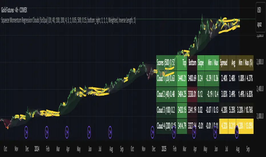
Squeeze Momentum Regression Clouds [SciQua]╭──────────────────────────────────────────────╮
☁️ Squeeze Momentum Regression Clouds
╰──────────────────────────────────────────────╯
🔍 Overview
The Squeeze Momentum Regression Clouds (SMRC) indicator is a powerful visual tool for identifying price compression , trend strength , and slope momentum using multiple layers of linear regression Clouds. Designed to extend the classic squeeze framework, this indicator captures the behavior of price through dynamic slope detection, percentile-based spread analytics, and an optional UI for trend inspection — across up to four customizable regression Clouds .
────────────────────────────────────────────────────────────
╭────────────────╮
⚙️ Core Features
╰────────────────╯
Up to 4 Regression Clouds – Each Cloud is created from a top and bottom linear regression line over a configurable lookback window.
Slope Detection Engine – Identifies whether each band is rising, falling, or flat based on slope-to-ATR thresholds.
Spread Compression Heatmap – Highlights compressed zones using yellow intensity, derived from historical spread analysis.
Composite Trend Scoring – Aggregates directional signals from each Cloud using your chosen weighting model.
Color-Coded Candles – Optional candle coloring reflects the real-time composite score.
UI Table – A toggleable info table shows slopes, compression levels, percentile ranks, and direction scores for each Cloud.
Gradient Cloud Styling – Apply gradient coloring from Cloud 1 to Cloud 4 for visual slope intensity.
Weight Aggregation Options – Use equal weighting, inverse-length weighting, or max pooling across Clouds to determine composite trend strength.
────────────────────────────────────────────────────────────
╭──────────────────────────────────────────╮
🧪 How to Use the Indicator
1. Understand Trend Bias with Cloud Colors
╰──────────────────────────────────────────╯
Each Cloud changes color based on its current slope:
Green indicates a rising trend.
Red indicates a falling trend.
Gray indicates a flat slope — often seen during chop or transitions.
Cloud 1 typically reflects short-term structure, while Cloud 4 represents long-term directional bias. Watch for multi-Cloud alignment — when all Clouds are green or red, the trend is strong. Divergence among Clouds often signals a potential shift.
────────────────────────────────────────────────────────────
╭───────────────────────────────────────────────╮
2. Use Compression Heat to Anticipate Breakouts
╰───────────────────────────────────────────────╯
The space between each Cloud’s top and bottom regression lines is measured, normalized, and analyzed over time. When this spread tightens relative to its history, the script highlights the band with a yellow compression glow .
This visual cue helps identify squeeze zones before volatility expands. If you see compression paired with a changing slope color (e.g., gray to green), this may indicate an impending breakout.
────────────────────────────────────────────────────────────
╭─────────────────────────────────╮
3. Leverage the Optional Table UI
╰─────────────────────────────────╯
The indicator includes a dynamic, floating table that displays real-time metrics per Cloud. These include:
Slope direction and value , with historical Min/Max reference.
Top and Bottom percentile ranks , showing how price sits within the Cloud range.
Current spread width , compared to its historical norms.
Composite score , which blends trend, slope, and compression for that Cloud.
You can customize the table’s position, theme, transparency, and whether to show a combined summary score in the header.
────────────────────────────────────────────────────────────
╭─────────────────────────────────────────────╮
4. Analyze Candle Color for Composite Signals
╰─────────────────────────────────────────────╯
When enabled, the indicator colors candles based on a weighted composite score. This score factors in:
The signed slope of each Cloud (up, down, or flat)
The percentile pressure from the top and bottom bands
The degree of spread compression
Expect green candles in bullish trend phases, red candles during bearish regimes, and gray candles in mixed or low-conviction zones.
Candle coloring provides a visual shorthand for market conditions , useful for intraday scanning or historical backtesting.
────────────────────────────────────────────────────────────
╭────────────────────────╮
🧰 Configuration Guidance
╰────────────────────────╯
To tailor the indicator to your strategy:
Use Cloud lengths like 21, 34, 55, and 89 for a balanced multi-timeframe view.
Adjust the slope threshold (default 0.05) to control how sensitive the trend coloring is.
Set the spread floor (e.g., 0.15) to tune when compression is detected and visualized.
Choose your weighting style : Inverse Length (favor faster bands), Equal, or Max Pooling (most aggressive).
Set composite weights to emphasize trend slope, percentile bias, or compression—depending on your market edge.
────────────────────────────────────────────────────────────
╭────────────────╮
✅ Best Practices
╰────────────────╯
Use aligned Cloud colors across all bands to confirm trend conviction.
Combine slope direction with compression glow for early breakout entry setups.
In choppy markets, watch for Clouds 1 and 2 turning flat while Clouds 3 and 4 remain directional — a sign of potential trend exhaustion or consolidation.
Keep the table enabled during backtesting to manually evaluate how each Cloud behaved during price turns and consolidations.
────────────────────────────────────────────────────────────
╭───────────────────────╮
📌 License & Usage Terms
╰───────────────────────╯
This script is provided under the Creative Commons Attribution-NonCommercial 4.0 International License .
✅ You are allowed to:
Use this script for personal or educational purposes
Study, learn, and adapt it for your own non-commercial strategies
❌ You are not allowed to:
Resell or redistribute the script without permission
Use it inside any paid product or service
Republish without giving clear attribution to the original author
For commercial licensing , private customization, or collaborations, please contact Joshua Danford directly.
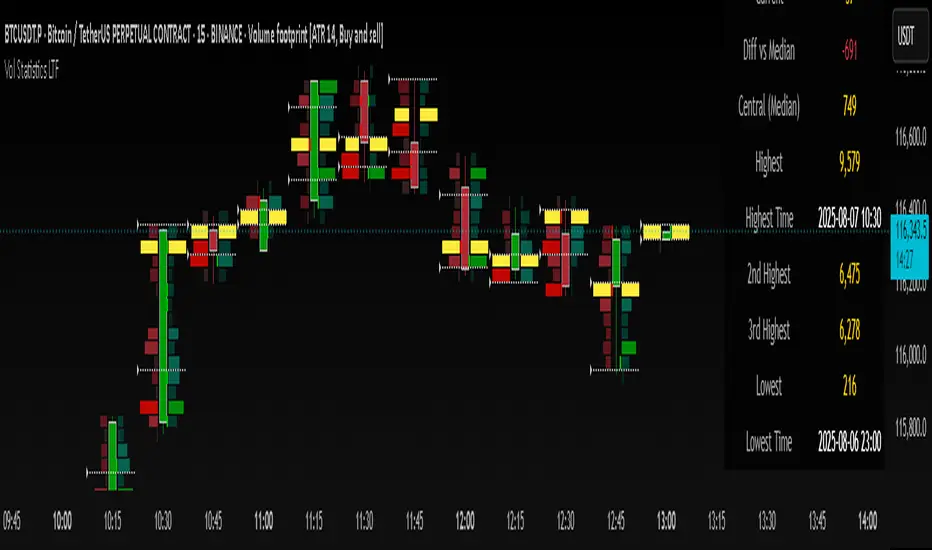
Volume Statistics - IntraweekVolume Statistics - Intraweek: For Orderflow Traders
This tool is designed for traders using volume footprint charts and orderflow methods.
Why it matters:
In orderflow trading, you care about the quality of volume behind each move. You’re not just watching price; you’re watching how much aggression is behind that price move. That’s where this indicator helps.
What to look at:
* Current Volume shows you how much volume is trading right now.
* Central Volume (median or average over 24h or 7D) gives you a baseline for what's normal volume VS abnormal volume.
* The Diff vs Central tells you immediately if current volume is above or below normal.
How this helps:
* If volume is above normal, it suggested elevated levels of buyer or seller aggression. Look for strong follow-through or continuation.
* If volume is below normal, it may signal low interest, passive participation, a lack of conviction, or a fake move.
* Use this context to decide if what you're seeing in the footprint (imbalances, absorption, traps) is actually worth acting on.
Extra context:
* The highest and lowest volume levels and their timestamps help you spot prior key reactions.
* Second and third highest bars help you see other major effort points in the recent window.
Comment with any suggestions on how to improve this indicator.
ACR(Average Candle Range) With TargetsWhat is ACR?
The Average Candle Range (ACR) is a custom volatility metric that calculates the mean distance between the high and low of a set number of past candles. ACR focuses only on the actual candle range (high - low) of specific past candles on a chosen timeframe.
This script calculates and visualizes the Average Candle Range (ACR) over a user-defined number of candles on a custom timeframe. It displays a table of recent range values, plots dynamic bullish and bearish target levels, and marks the start of each new candle with a vertical line. All calculations update in real time as price action develops. This script was inspired by the “ICT ADR Levels - Judas x Daily Range Meter°” by toodegrees.
Key Features
Custom Timeframe Selection: Choose any timeframe (e.g., 1D, 4H, 15m) for analysis.
User-Defined Lookback: Calculate the average range across 1 to 10 previous candles.
Dynamic Targets:
Bullish Target: Current candle low + ACR.
Bearish Target: Current candle high – ACR.
Live Updates: Targets adjust intrabar as highs or lows change during the current candle.
Candle Start Markers: Vertical lines denote the open of each new candle on the selected timeframe.
Floating Range Table:
Displays the current ACR value.
Lists individual ranges for the previous five candles.
Extend Target Lines: Choose to extend bullish and bearish target levels fully across the screen.
Global Visibility Controls: Toggle on/off all visual elements (targets, vertical lines, and table) for a cleaner view.
How It Works
At each new candle on the user-selected timeframe, the script:
Draws a vertical line at the candle’s open.
Recalculates the ACR based on the inputted previous number of candles.
Plots target levels using the current candle's developing high and low values.
Limitation
Once the price has already moved a full ACR in the opposite direction from your intended trade, the associated target loses its practical value. For example, if you intended to trade long but the bearish ACR target is hit first, the bullish target is no longer a reliable reference for that session.
Use Case
This tool is designed for traders who:
Want to visualize the average movement range of candles over time.
Use higher or lower timeframe candles as structural anchors.
Require real-time range-based price levels for intraday or swing decision-making.
This script does not generate entry or exit signals. Instead, it supports range awareness and target projection based on historical candle behavior.
Key Difference from Similar Tools
While this script was inspired by “ICT ADR Levels - Judas x Daily Range Meter°” by toodegrees, it introduces a major enhancement: the ability to customize the timeframe used for calculating the range. Most ADR or candle-range tools are locked to a single timeframe (e.g., daily), but this version gives traders full control over the analysis window. This makes it adaptable to a wide range of strategies, including intraday and swing trading, across any market or asset.
