Time-Based Fair Value Gaps (FVG) with Inversions (iFVG)Overview
The Time-Based Fair Value Gaps (FVG) with Inversions (iFVG) (ICT/SMT) indicator is a specialized tool designed for traders using Inner Circle Trader (ICT) methodologies. Inspired by LuxAlgo's Fair Value Gap indicator, this script introduces significant enhancements by integrating ICT principles, focusing on precise time-based FVG detection, inversion tracking, and retest signals tailored for institutional trading strategies. Unlike LuxAlgo’s general FVG approach, this indicator filters FVGs within customizable 10-minute windows aligned with ICT’s macro timeframes and incorporates ICT-specific concepts like mitigation, liquidity grabs, and session-based gap prioritization.
This tool is optimized for 1–5 minute charts, though probably best for 1 minute charts, identifying bullish and bearish FVGs, tracking their mitigation into inverted FVGs (iFVGs) as key support/resistance zones, and generating retest signals with customizable “Close” or “Wick” confirmation. Features like ATR-based filtering, optional FVG labels, mitigation removal, and session-specific FVG detection (e.g., first FVG in AM/PM sessions) make it a powerful tool for ICT traders.
Originality and Improvements
While inspired by LuxAlgo’s FVG indicator (credit to LuxAlgo for their foundational work), this script significantly extends the original concept by:
1. Time-Based FVG Detection: Unlike LuxAlgo’s continuous FVG identification, this script filters FVGs within user-defined 10-minute windows each hour (:00–:10, :10–:20, etc.), aligning with ICT’s emphasis on specific periods of institutional activity, such as hourly opens/closes or kill zones (e.g., New York 7:00–11:00 AM EST). This ensures FVGs are relevant to high-probability ICT setups.
2. Session-Specific First FVG Option: A unique feature allows traders to display only the first FVG in ICT-defined AM (9:30–10:00 AM EST) or PM (1:30–2:00 PM EST) sessions, reflecting ICT’s focus on initial market imbalances during key liquidity events.
3. ICT-Driven Mitigation and Inversion Logic: The script tracks FVG mitigation (when price closes through a gap) and converts mitigated FVGs into iFVGs, which serve as ICT-style support/resistance zones. This aligns with ICT’s view that mitigated gaps become critical reversal points, unlike LuxAlgo’s simpler gap display.
4. Customizable Retest Signals: Retest signals for iFVGs are configurable for “Close” (conservative, requiring candle body confirmation) or “Wick” (faster, using highs/lows), catering to ICT traders’ need for precise entry timing during liquidity grabs or Judas swings.
5. ATR Filtering and Mitigation Removal: An optional ATR filter ensures only significant FVGs are displayed, reducing noise, while mitigation removal declutters the chart by removing filled gaps, aligning with ICT’s principle that mitigated gaps lose relevance unless inverted.
6. Timezone and Timeframe Safeguards: A timezone offset setting aligns FVG detection with EST for ICT’s New York-centric strategies, and a timeframe warning alerts users to avoid ≥1-hour charts, ensuring accuracy in time-based filtering.
These enhancements make the script a distinct tool that builds on LuxAlgo’s foundation while offering ICT traders a tailored, high-precision solution.
How It Works
FVG Detection
FVGs are identified when a candle’s low is higher than the high of two candles prior (bullish FVG) or a candle’s high is lower than the low of two candles prior (bearish FVG). Detection is restricted to:
• User-selected 10-minute windows (e.g., :00–:10, :50–:60) to capture ICT-relevant periods like hourly transitions.
• AM/PM session first FVGs (if enabled), focusing on 9:30–10:00 AM or 1:30–2:00 PM EST for key market opens.
An optional ATR filter (default: 0.25× ATR) ensures only gaps larger than the threshold are displayed, prioritizing significant imbalances.
Mitigation and Inversion
When price closes through an FVG (e.g., below a bullish FVG’s bottom), the FVG is mitigated and becomes an iFVG, plotted as a support/resistance zone. iFVGs are critical in ICT for identifying reversal points where institutional orders accumulate.
Retest Signals
The script generates signals when price retests an iFVG:
• Close: Triggers when the candle body confirms the retest (conservative, lower noise).
• Wick: Triggers when the candle’s high/low touches the iFVG (faster, higher sensitivity). Signals are visualized with triangular markers (▲ for bullish, ▼ for bearish) and can trigger alerts.
Visualization
• FVGs: Displayed as colored boxes (green for bullish, red for bearish) with optional “Bull FVG”/“Bear FVG” labels.
• iFVGs: Shown as extended boxes with dashed midlines, limited to the user-defined number of recent zones (default: 5).
• Mitigation Removal: Mitigated FVGs/iFVGs are removed (if enabled) to keep the chart clean.
How to Use
Recommended Settings
• Timeframe: Use 1–5 minute charts for precision, avoiding ≥1-hour timeframes (a warning label appears if misconfigured).
• Time Windows: Enable :00–:10 and :50–:60 for hourly open/close FVGs, or use the “Show only 1st presented FVG” option for AM/PM session focus.
• ATR Filter: Keep enabled (multiplier 0.25–0.5) for significant gaps; disable on 1-minute charts for more FVGs during volatility.
• Signal Preference: Use “Close” for conservative entries, “Wick” for aggressive setups.
• Timezone Offset: Set to -5 for EST (or -4 for EDT) to align with ICT’s New York session.
Trading Strategy
1. Macro Timeframes: Focus on New York (7:00–11:00 AM EST) or London (2:00–5:00 AM EST) kill zones for high institutional activity.
2. FVG Entries: Trade bullish FVGs as support in uptrends or bearish FVGs as resistance in downtrends, especially in :00–:10 or :50–:60 windows.
3. iFVG Retests: Enter on retest signals (▲/▼) during liquidity grabs or Judas swings, using “Close” for confirmation or “Wick” for speed.
4. Session FVGs: Use the “Show only 1st presented FVG” option to target the first gap in AM/PM sessions, often tied to ICT’s market maker algorithms.
5. Risk Management: Combine with ICT concepts like order blocks or breaker blocks for confluence, and set stops beyond FVG/iFVG boundaries.
Alerts
Set alerts for:
• “Bullish FVG Detected”/“Bearish FVG Detected”: New FVGs in selected windows.
• “Bullish Signal”/“Bearish Signal”: iFVG retest confirmations.
Settings Description
• Show Last (1–100, default: 5): Number of recent iFVGs to display. Lower values reduce clutter.
• Show only 1st presented FVG : Limits FVGs to the first in 9:30–10:00 AM or 1:30–2:00 PM EST sessions (overrides time window checkboxes).
• Time Window Checkboxes: Enable/disable FVG detection in 10-minute windows (:00–:10, :10–:20, etc.). All enabled by default.
• Signal Preference: “Close” (default) or “Wick” for iFVG retest signals.
• Use ATR Filter: Enables ATR-based size filtering (default: true).
• ATR Multiplier (0–∞, default: 0.25): Sets FVG size threshold (higher values = larger gaps).
• Remove Mitigated FVGs: Removes filled FVGs/iFVGs (default: true).
• Show FVG Labels: Displays “Bull FVG”/“Bear FVG” labels (default: true).
• Timezone Offset (-12 to 12, default: -5): Aligns time windows with EST.
• Colors: Customize bullish (green), bearish (red), and midline (gray) colors.
Why Use This Indicator?
This indicator empowers ICT traders with a tool that goes beyond generic FVG detection, offering precise, time-filtered gaps and inversion tracking aligned with institutional trading principles. By focusing on ICT’s macro timeframes, session-specific imbalances, and customizable signal logic, it provides a clear edge for scalping, swing trading, or reversal setups in high-liquidity markets.
在腳本中搜尋"市值60亿的股票"
Green*DiamondGreen*Diamond (GD1)
Unleash Dynamic Trading Signals with Volatility and Momentum
Overview
GreenDiamond is a versatile overlay indicator designed for traders seeking actionable buy and sell signals across various markets and timeframes. Combining Volatility Bands (VB) bands, Consolidation Detection, MACD, RSI, and a unique Ribbon Wave, it highlights high-probability setups while filtering out noise. With customizable signals like Green-Yellow Buy, Pullback Sell, and Inverse Pullback Buy, plus vibrant candle and volume visuals, GreenDiamond adapts to your trading style—whether you’re scalping, day trading, or swing trading.
Key Features
Volatility Bands (VB): Plots dynamic upper and lower bands to identify breakouts or reversals, with toggleable buy/sell signals outside consolidation zones.
Consolidation Detection: Marks low-range periods to avoid choppy markets, ensuring signals fire during trending conditions.
MACD Signals: Offers flexible buy/sell conditions (e.g., cross above signal, above zero, histogram up) with RSI divergence integration for precision.
RSI Filter: Enhances signals with customizable levels (midline, oversold/overbought) and bullish divergence detection.
Ribbon Wave: Visualizes trend strength using three EMAs, colored by MACD and RSI for intuitive momentum cues.
Custom Signals: Includes Green-Yellow Buy, Pullback Sell, and Inverse Pullback Buy, with limits on consecutive signals to prevent overtrading.
Candle & Volume Styling: Blends MACD/RSI colors on candles and scales volume bars to highlight momentum spikes.
Alerts: Set up alerts for VB signals, MACD crosses, Green*Diamond signals, and custom conditions to stay on top of opportunities.
How It Works
Green*Diamond integrates multiple indicators to generate signals:
Volatility Bands: Calculates bands using a pivot SMA and standard deviation. Buy signals trigger on crossovers above the lower band, sell signals on crossunders below the upper band (if enabled).
Consolidation Filter: Suppresses signals when candle ranges are below a threshold, keeping you out of flat markets.
MACD & RSI: Combines MACD conditions (e.g., cross above signal) with RSI filters (e.g., above midline) and optional volume spikes for robust signals.
Custom Logic: Green-Yellow Buy uses MACD bullishness, Pullback Sell targets retracements, and Inverse Pullback Buy catches reversals after downmoves—all filtered to avoid consolidation.
Visuals: Ribbon Wave shows trend direction, candles blend momentum colors, and volume bars scale dynamically to confirm signals.
Settings
Volatility Bands Settings:
VB Lookback Period (20): Adjust to 10–15 for faster markets (e.g., 1-minute scalping) or 25–30 for daily charts.
Upper/Lower Band Multiplier (1.0): Increase to 1.5–2.0 for wider bands in volatile stocks like AEHL; decrease to 0.5 for calmer markets.
Show Volatility Bands: Toggle off to reduce chart clutter.
Use VB Signals: Enable for breakout-focused trades; disable to focus on Green*Diamond signals.
Consolidation Settings:
Consolidation Lookback (14): Set to 5–10 for small caps (e.g., AEHL) to catch quick consolidations; 20 for higher timeframes.
Range Threshold (0.5): Lower to 0.3 for stricter filtering in choppy markets; raise to 0.7 for looser signals.
MACD Settings:
Fast/Slow Length (12/26): Shorten to 8/21 for scalping; extend to 15/34 for swing trading.
Signal Smoothing (9): Reduce to 5 for faster signals; increase to 12 for smoother trends.
Buy/Sell Signal Options: Choose “Cross Above Signal” for classic MACD; “Histogram Up” for momentum plays.
Use RSI Div + MACD Cross: Enable for high-probability reversal signals.
RSI Settings:
RSI Period (14): Drop to 10 for 1-minute charts; raise to 20 for daily.
Filter Level (50): Set to 55 for stricter buys; 45 for sells.
Overbought/Oversold (70/30): Tighten to 65/35 for small caps; widen to 75/25 for indices.
RSI Buy/Sell Options: Select “Bullish Divergence” for reversals; “Cross Above Oversold” for momentum.
Color Settings:
Adjust bullish/bearish colors for visibility (e.g., brighter green/red for dark themes).
Border Thickness (1): Increase to 2–3 for clearer candle outlines.
Volume Settings:
Volume Average Length (20): Shorten to 10 for scalping; extend to 30 for swing trades.
Volume Multiplier (2.0): Raise to 3.0 for AEHL’s volume surges; lower to 1.5 for steady stocks.
Bar Height (10%): Increase to 15% for prominent bars; decrease to 5% to reduce clutter.
Ribbon Settings:
EMA Periods (10/20/30): Tighten to 5/10/15 for scalping; widen to 20/40/60 for trends.
Color by MACD/RSI: Disable for simpler visuals; enable for dynamic momentum cues.
Gradient Fill: Toggle on for trend clarity; off for minimalism.
Custom Signals:
Enable Green-Yellow Buy: Use for momentum confirmation; limit to 1–2 signals to avoid spam.
Pullback/Inverse Pullback % (50): Set to 30–40% for small caps; 60–70% for indices.
Max Buy Signals (1): Increase to 2–3 for active markets; keep at 1 for discipline.
Tips and Tricks
Scalping Small Caps (e.g., AEHL):
Use 1-minute charts with VB Lookback = 10, Consolidation Lookback = 5, and Volume Multiplier = 3.0 to catch $0.10–$0.20 moves.
Enable Green-Yellow Buy and Inverse Pullback Buy for quick entries; disable VB Signals to focus on Green*Diamond logic.
Pair with SMC+ green boxes (if you use them) for reversal confirmation.
Day Trading:
Try 5-minute charts with MACD Fast/Slow = 8/21 and RSI Period = 10.
Enable RSI Divergence + MACD Cross for high-probability setups; set Max Buy Signals = 2.
Watch for volume bars turning yellow to confirm entries.
Swing Trading:
Use daily charts with VB Lookback = 30, Ribbon EMAs = 20/40/60.
Enable Pullback Sell (60%) to exit after rallies; disable RSI Color for cleaner candles.
Check Ribbon Wave gradient for trend strength—bright green signals strong bulls.
Avoiding Noise:
Increase Consolidation Threshold to 0.7 on volatile days to skip false breakouts.
Disable Ribbon Wave or Volume Bars if the chart feels crowded.
Limit Max Buy Signals to 1 for disciplined trading.
Alert Setup:
In TradingView’s Alerts panel, select:
“GD Buy Signal” for standard entries.
“RSI Div + MACD Cross Buy” for reversals.
“VB Buy Signal” for breakout plays.
Set to “Once Per Bar Close” for confirmed signals; “Once Per Bar” for scalping.
Backtesting:
Replay on small caps ( Float < 5M, Price $0.50–$5) to test signals.
Focus on “GD Buy Signal” with yellow volume bars and green Ribbon Wave.
Avoid signals during gray consolidation squares unless paired with RSI Divergence.
Usage Notes
Markets: Works on stocks, forex, crypto, and indices. Best for volatile assets (e.g., small-cap stocks, BTCUSD).
Timeframes: Scalping (1–5 minutes), day trading (15–60 minutes), or swing trading (daily). Adjust settings per timeframe.
Risk Management: Combine with stop-losses (e.g., 1% risk, $0.05 below AEHL entry) and take-profits (3–5%).
Customization: Tweak inputs to match your strategy—experiment in replay to find your sweet spot.
Disclaimer
Green*Diamond is a technical tool to assist with trade identification, not a guarantee of profits. Trading involves risks, and past performance doesn’t predict future results. Always conduct your own analysis, manage risk, and test settings before live trading.
Feedback
Love Green*Diamond? Found a killer setup?

Mercury Venus Conjunction Sextiles 2019-2026How to Use It and What It Means Astrologically
How to Use the Script in TradingView
This Pine Script, called "Mercury Venus Aspects 2019–2026," is made to highlight the dates of Mercury-Venus conjunctions (0°) and sextiles (60°) from 2019 to 2026 on TradingView charts. Here's how to use it:
click “Add to Chart.” It will apply to any chart you have open—stocks, forex, crypto, etc.
Customize the Display
You can turn on/off the visibility of conjunctions and sextiles using checkboxes under "Inputs" in the settings.
You can also adjust the label size (small, normal, large, or huge) for better readability on your chart.
What You’ll See on the Chart
Conjunctions appear as blue shaded zones with labels like “C1,” “C2,” etc. These mark dates when Mercury and Venus are at the same degree.
Sextiles show up in orange with labels like “S1,” “S2,” marking when they’re about 60° apart.
Each event spans a 2-day window (one day before and after the exact aspect).
How to Use It Practically
You can overlay the script on market charts to look for any patterns between these planetary aspects and price movements.
You can also use it to plan personal or financial activities, since these aspects often affect communication, money, and relationships.
What to Keep in Mind
Dates are approximate and based on average planetary cycles (Mercury: ~88 days, Venus: ~225 days). For exact timing, use an ephemeris.
Only conjunctions and sextiles are shown. Oppositions, squares, and trines aren’t included because Mercury and Venus never get far enough apart (more than 75°).
This script is great for astrologers, traders, and enthusiasts who want to see Mercury-Venus aspects directly on their charts and explore their possible effects.
Astrological Meaning of Mercury-Venus Aspects
What Mercury and Venus Represent
Mercury rules communication, thinking, technology, travel, and trade. In global events (mundane astrology), it affects media, markets, and movement of information.
Venus is about love, beauty, money, and pleasure. It influences relationships, aesthetics, and finance. In the world stage, it’s linked to luxury, art, fashion, and economic balance.
When Mercury and Venus form aspects (like conjunctions or sextiles), their energies mix in helpful ways that can affect people and events.
Conjunction (0°) – Mercury and Venus Together
These two planets are in the same sign and degree, so their qualities merge.
For people:
Positive: Smooth communication, charm, creativity, and better relationships. Great for romance, art, and social interaction.
Negative: Too much focus on appearances, sweet talk, or pleasure can cloud judgment. Decisions may lack depth.
For the economy:
Positive: Boosts in media, entertainment, fashion, and tech. Good for trade, deals, and optimism in financial markets.
Negative: Risk of overspending or unrealistic expectations. May cause small market bubbles or misleading hype.
Sextile (60°) – Mercury and Venus in Harmony
These two planets are two signs apart, creating a smooth, supportive energy.
For people:
Positive: Easy conversations, creative teamwork, small financial wins, and pleasant social experiences.
Negative: Energy is mild, so opportunities might be missed if not acted on. People may avoid hard decisions.
For the economy:
Positive: Gradual improvements in areas like marketing, social media, hospitality, and design. Good for diplomacy.
Negative: Lack of strong initiative could limit bigger gains. Minor missteps are possible due to a laid-back attitude.
General Effects
These aspects are mostly beneficial. They support creativity, financial thinking, and social harmony.
Downsides: Conjunctions may lead to overindulgence or shallow choices, while sextiles may cause missed chances due to low energy.
These aspects rarely cause major economic shifts on their own but can amplify trends depending on other planetary influences (like Saturn or Uranus).
Zodiac Sign Influence
Fire signs (Aries, Leo, Sagittarius): Bold communication, energetic spending, gains in media or entertainment.
Earth signs (Taurus, Virgo, Capricorn): Practical results, stable finances, growth in real-world assets like property or food.
Air signs (Gemini, Libra, Aquarius): Intellectual growth, tech innovation, and social ideas flourish.
Water signs (Cancer, Scorpio, Pisces): Emotional depth in conversations, artistic growth, and financial sensitivity.
Mercury-Venus aspects are gentle but helpful. They combine logic (Mercury) with emotion and value (Venus). They’re good times for love, communication, and money—but their benefits depend on how we use the energy. This script lets you easily track these moments on a chart and explore how they might align with real-life trends or decisions.
Disclaimer: This script and its interpretations are for informational and educational purposes only. They do not constitute financial, trading, or professional astrological advice. Always conduct your own research and consult qualified professionals before making any financial or personal decisions. Use at your own discretion.

Dskyz Adaptive Futures Elite (DAFE)Dskyz Adaptive Futures Edge (DAFE)
imgur.com
A Dynamic Futures Trading Strategy
DAFE adapts to market volatility and price action using technical indicators and advanced risk management. It’s built for high-stakes futures trading (e.g., MNQ, BTCUSDT.P), offering modular logic for scalpers and swing traders alike.
Key Features
Adaptive Moving Averages
Dynamic Logic: Fast and slow SMAs adjust lengths via ATR, reacting to momentum shifts and smoothing in calm markets.
Signals: Long entry on fast SMA crossing above slow SMA with price confirmation; short on cross below.
RSI Filtering (Optional)
Momentum Check: Confirms entries with RSI crossovers (e.g., above oversold for longs). Toggle on/off with custom levels.
Fine-Tuning: Adjustable lookback and thresholds (e.g., 60/40) for precision.
Candlestick Pattern Recognition
Eng|Enhanced Detection: Identifies strong bullish/bearish engulfing patterns, validated by volume and range strength (vs. 10-period SMA).
Conflict Avoidance: Skips trades if both patterns appear in the lookback window, reducing whipsaws.
Multi-Timeframe Trend Filter
15-Minute Alignment: Syncs intrabar trades with 15-minute SMA trends; optional for flexibility.
Dollar-Cost Averaging (DCA) New!
Scaling: Adds up to a set number of entries (e.g., 4) on pullbacks/rallies, spaced by ATR multiples.
Control: Caps exposure and resets on exit, enhancing trend-following potential.
Trade Execution & Risk Management
Entry Rules: Prioritizes moving averages or patterns (user choice), with volume, volatility, and time filters.
Stops & Trails:
Initial Stop: ATR-based (2–3.5x, volatility-adjusted).
Trailing Stop: Locks profits with configurable ATR offset and multiplier.
Discipline
Cooldown: Pauses post-exit (e.g., 0–5 minutes).
Min Hold: Ensures trades last a set number of bars (e.g., 2–10).
Visualization & Tools
Charts: Overlays MAs, stops, and signals; trend shaded in background.
Dashboard: Shows position, P&L, win rate, and more in real-time.
Debugging: Logs signal details for optimization.
Input Parameters
Parameter Purpose Suggested Use
Use RSI Filter - Toggle RSI confirmation *Disable 4 price-only
trading
RSI Length - RSI period (e.g., 14) *7–14 for sensitivity
RSI Overbought/Oversold - Adjust for market type *Set levels (e.g., 60/40)
Use Candlestick Patterns - Enables engulfing signals *Disable for MA focus
Pattern Lookback - Pattern window (e.g., 19) *10–20 bars for balance
Use 15m Trend Filter - Align with 15-min trend *Enable for trend trades
Fast/Slow MA Length - Base MA lengths (e.g., 9/19) *10–25 / 30–60 per
timeframe
Volatility Threshold - Filters volatile spikes *Max ATR/close (e.g., 1%)
Min Volume - Entry volume threshold *Avoid illiquid periods
(e.g., 10)
ATR Length - ATR period (e.g., 14) *Standard volatility
measure
Trailing Stop ATR Offset - Trail distance (e.g., 0.5) *0.5–1.5 for tightness
Trailing Stop ATR Multi - Trail multiplier (e.g., 1.0) *1–3 for trend room
Cooldown Minutes - Post-exit pause (e.g., 0–5) *Prevents overtrading
Min Bars to Hold - Min trade duration (e.g., 2) *5–10 for intraday
Trading Hours - Active window (e.g., 9–16) *Focus on key sessions
Use DCA - Toggle DCA *Enable for scaling
Max DCA Entries - Cap entries (e.g., 4) *Limit risk exposure
DCA ATR Multiplier Entry spacing (e.g., 1.0) *1–2 for wider gaps
Compliance
Realistic Testing: Fixed quantities, capital, and slippage for accurate backtests.
Transparency: All logic is user-visible and adjustable.
Risk Controls: Cooldowns, stops, and hold periods ensure stability.
Flexibility: Adapts to various futures and timeframes.
Summary
DAFE excels in volatile futures markets with adaptive logic, DCA scaling, and robust risk tools. Currently in prop account testing, it’s a powerful framework for precision trading.
Caution
DAFE is experimental, not a profit guarantee. Futures trading risks significant losses due to leverage. Backtest, simulate, and monitor actively before live use. All trading decisions are your responsibility.

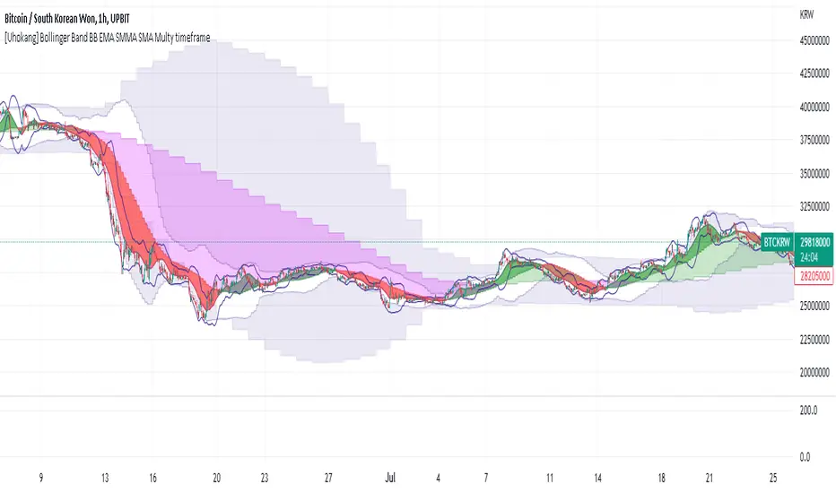
Statistical OHLC Projections [neo|]█ OVERVIEW
Statistical OHLC Projections is an indicator designed to offer users a customizable deep-dive on measuring historical price levels for any timeframe. The indicator separates price into two distinct levels, "Manipulation" and "Distribution", where the idea is that for higher timeframe candles, e.g. an up-close candle, the distance from the open to the bottom of the wick would constitute the Manipulation, and the rest would be considered the Distribution. By measuring out these levels, we can gain insight on how far the market may move from higher timeframe opens to their manipulations and distributions, and apply this knowledge to our analysis.
IMPORTANT: Since levels are based on the lookback available on your chart, if the levels aren't being displayed this likely means you don't have enough lookback for your selected timeframe. To check this, enable the stat table to see how many values are available for your timeframe, and either reduce the lookback or increase your chart timeframe.
█ CONCEPTS
The core concept revolves around understanding market behavior through the lens of historical candle structure. The indicator dissects OHLC data to provide statistical boundaries of expected price movement.
- Manipulation Levels: These represent the areas typically seen as liquidity grabs or false moves where price extends in one direction before reversing.
- Distribution Levels: These highlight where the bulk of directional movement tends to occur, often following the manipulation move.
The tool aggregates this data across your selected timeframe to inform you of potential levels associated with it.
█ FEATURES
Multiple Display Types: Display statistical data through two sleek styles, areas or lines. Where areas represent the area between two customizable lookback values, and lines represent one average value.
Adjustable Timeframe Selection: Whether you want to see data based on the 1D chart, or the 1W chart, anything is possible. Simply change the timeframe on the dropdown menu and if there is sufficient lookback the indicator will adjust to your requested timeframe.
Customizable Historical Lookback: By default, the indicator will measure the average 60 values of your requested timeframe, however this may be adjusted to be higher or lower based on your preference. If you want to measure recent moves, 10-20 lookback may be better for you, or if you want more data for less volatile instruments, a value of 100 may be better.
Historical Display: Prevent historical levels from being removed by unchecking the "Remove Previous Drawings" option, this will allow you to examine how the levels previously interacted with price.
NY Midnight Anchoring: By checking the "Use NY Midnight" option, you may see the projection anchored to the New York midnight open time, which is often a significant level on indices.
Alerts: You may enable alerts for any of the indicator's provided levels to stay informed, even when off the charts.
█ How to use
To use the indicator, simply apply it to your chart and modify any of your desired inputs.
By default, the indicator will provide levels for the "1D" timeframe, with a desired lookback of 60, on most instruments and plans this can be gotten when you are on the 30 minute timeframe or above.
When price reaches or extends beyond a manipulation level, observe how it reacts and whether it rejects from that level, if it does this may be an indication that the candle for the timeframe you selected may be reversing.
█ SETTINGS AND OPTIONS
Customize the indicator’s behavior, timeframe sources, and visual appearance to fit your analysis style. Each setting has been designed with flexibility in mind, whether you're working on lower or higher timeframes.
Display Mode: Switch between different display styles for levels: - Default: Shows all statistical levels as individual lines.
- Areas: Plots filled zones between two customizable lookbacks to represent the range between them.
This is ideal for visually mapping high-probability zones of price activity.
Timeframe Settings:
- Show First/Second Timeframe: Choose to show one or both timeframe projections simultaneously.
- First Timeframe / Second Timeframe: Define the higher timeframe candle you want to base calculations on (e.g., 1D, 1W).
- Use NY Midnight: When enabled and using the daily timeframe, the levels will be anchored to the New York Midnight Open (00:00 EST), a key institutional timing reference, especially useful for indices and forex.
Calculation Settings:
- Main Lookback Period: The number of historical candles used in the statistical calculations. A lower number focuses on recent price action, while a higher number smooths results across broader history.
- First Lookback / Second Lookback: Used when “Areas” mode is selected to define the range of the shaded zone. For example, an area from 20 to 60 candles creates a band between short- and long-term price behavior averages.
Visual Settings:
- Line Style: Set your preferred visual style: Solid, Dashed, or Dotted.
- Remove Previous Drawings: When enabled, only the most recent projection is shown on the chart. Disable to retain previous levels and visually backtest their reactions over time.
Color Settings:
Customize each level independently to match your chart theme:
- Manipulation High/Low
- Distribution High/Low
- Open Level
- Label Text Color
Premium/Discount Zones:
- Enable Premium/Discount Zones: Overlay price zones above and below equilibrium to visualize potential overbought (premium) and oversold (discount) areas.
- Premium/Discount Colors: Fully customizable zone colors for clarity and emphasis.
Table Settings:
- Show Statistics Table: Adds an on-chart table summarizing key levels from your active timeframe(s).
- Table Cell Color: Set the background color of the table cells for visibility.
- Table Position: Choose from preset chart locations to position the table where it works best for your layout.
Alerts:
Stay on top of price interactions with key levels even when you're away from the charts.
- Manipulation Hits (High)
- Manipulation Hits (Low)
- Distribution Hits (High)
- Distribution Hits (Low)

4 EMA with Two Timeframes and Supertrend by Natee L.Key Features:
Customizable Timeframes:
The script has two inputs (timeframe_1 and timeframe_2) where you can select the timeframes for the two sets of EMAs. For example, you could choose:
timeframe_1 = "60" for 1-hour (60-minute) EMAs.
timeframe_2 = "240" for 4-hour (240-minute) EMAs.
Four EMAs for Each Timeframe:
It calculates 4 EMAs for both the first timeframe (timeframe_1) and the second timeframe (timeframe_2).
Plotting:
The EMAs for timeframe 1 are plotted in solid colors (blue, red, green, and purple).
The EMAs for timeframe 2 are plotted with a transparent effect (using color.new), so they are visually distinct but less dominant than the first timeframe's EMAs.
How to Use:
The timeframe_1 and timeframe_2 inputs allow you to select any timeframes you prefer (e.g., "15", "30", "60", "D", "W", etc.).
The EMAs for both selected timeframes will be plotted, allowing for easy comparison between the two timeframes on the same chart.
Explanation of the Updates:
Supertrend Calculation:
The Supertrend is calculated using the ta.supertrend function, which requires two parameters:
multiplier: The multiplier used for the Average True Range (ATR) calculation.
atr_period: The period for the ATR (usually set to 14).
The supertrend variable represents the value of the Supertrend, and direction is a boolean value indicating whether the trend is up (green) or down (red).
Supertrend Plot:
The Supertrend is plotted on the chart using the plot() function. The color is determined by the direction variable:
Green if the trend is up.
Red if the trend is down.
The Supertrend line is drawn with a linewidth of 2 for visibility.
Inputs:
atr_period: The period used for the ATR calculation, typically 14.
multiplier: The multiplier for the ATR to determine the offset for the Supertrend line.
How It Works:
The 4 EMAs are calculated for both timeframes (timeframe_1 and timeframe_2), just like before.
The Supertrend is calculated based on the ATR and the multiplier parameters, and it's plotted on the main chart.
The Supertrend changes color based on the trend direction (green for an uptrend, red for a downtrend).
Customization:
You can adjust the ATR period and multiplier as needed via the input fields.
You can also adjust the timeframes (timeframe_1 and timeframe_2) for the EMAs.
This script now combines the 4 EMAs and Supertrend indicators for two different timeframes, giving you a powerful tool for trend analysis and crossover strategies.

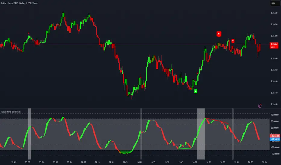
WaveTrend Divergences, Candle Colouring and TP Signal [LuciTech]WaveTrend is a momentum-based oscillator designed to track trend strength, detect divergences, and highlight potential take-profit zones using Bollinger Bands. It provides a clear visualization of market conditions to help traders identify trend shifts and exhaustion points.
The WaveTrend Oscillator consists of a smoothed momentum line (WT Line) and a signal line, which work together to indicate trend direction and possible reversals. When the WT Line crosses above the signal line, it suggests bullish momentum, while crossing below signals bearish momentum.
Candle colouring changes dynamically based on WaveTrend crossovers. If the WT Line crosses above the signal line, candles turn bullish. If the WT Line crosses below the signal line, candles turn bearish. This provides an immediate visual cue for trend direction.
Divergence Detection identifies when price action contradicts the WaveTrend movement.
Bullish Divergence appears when price makes a lower low, but the WT Line forms a higher low, suggesting weakening bearish pressure.
Bearish Divergence appears when price makes a higher high, but the WT Line forms a lower high, indicating weakening bullish pressure.
Plus (+) Divergences are stronger signals that occur when the first pivot of the divergence happens at an extreme level—above +60 for bearish divergence or below -60 for bullish divergence. These levels suggest the market is overbought or oversold, making the divergence more significant.
Bollinger Band Signals highlight potential take-profit zones by detecting when the WT Line moves beyond its upper or lower Bollinger Band.
If the WT Line crosses above the upper band, it signals stretched bullish momentum, suggesting a possible pullback or reversal.
If the WT Line crosses below the lower band, it indicates stretched bearish momentum, warning of a potential bounce.
How It Works
The WaveTrend momentum calculation is based on an EMA-smoothed moving average to filter out noise and provide a more reliable trend indication.
The WT Line (momentum line) fluctuates based on market momentum.
The signal line smooths out the WT Line to help identify trend shifts.
When the WT Line crosses above the signal line, it suggests buying pressure, and when it crosses below, it indicates selling pressure.
Divergences are detected by comparing pivot highs and lows in price with pivot highs and lows in the WT Line.
A pivot forms when a local high or low is confirmed after a certain number of bars.
The indicator tracks whether price action and the WT Line are making opposite movements.
If a divergence occurs and the first pivot was beyond ±60, it is marked as a Plus Divergence, making it a stronger reversal signal.
Bollinger Bands are applied directly to the WT Line instead of price, identifying when the WT Line moves outside its volatility range. This helps traders recognize when momentum is overstretched and a potential reversal or retracement is likely.
Settings
Channel Length (default: 8) controls the period used to calculate the WT Line.
Average Length (default: 16) smooths the WT Line for better trend detection.
Divergences (on/off) enables or disables divergence plotting.
Candle colouring (on/off) applies or removes trend-based candle colour changes.
Bollinger Band Signals (on/off) toggles take-profit signals when the WT Line crosses the bands.
Bullish/Bearish colours allow customization of divergence and signal colours.
Interpretation
The WaveTrend Oscillator helps traders assess market momentum and trend strength.
Crossovers between the WT Line and signal line indicate potential trend reversals.
Divergences warn of weakening momentum and possible reversals, with Plus Divergences acting as stronger signals.
Bollinger Band Crosses highlight areas where momentum is overstretched, signaling potential profit-taking opportunities.
UM VIX status table and Roll Yield with EMA
Description :
This oscillator indicator gives you a quick snapshot of VIX, VIX futures prices, and the related VIX roll yield at a glance. When the roll yield is greater than 0, The front-month VX1 future contract is less than the next-month VX2 contract. This is called Contango and is typical for the majority of the time. If the roll yield falls below zero. This is considered backwardation where the front-month VX1 contract is higher than the value of the next-month VX2 contract. Contango is most common. When Backwardation occurs, there is usually high volatility present.
Features :
The red and green fill indicate the current roll yield with the gray line being zero.
An Exponential moving average is overlaid on the roll yield. It is red when trending down and green when trending up. If you right-click the indicator, you can set alerts for roll yield EMA color transitions green to red or red to green.
Suggested uses:
The author suggests a one hour chart using the 55 period EMA with a 60 minute setting in the indicator. This gives you a visual idea of whether the roll yield is rising or falling. The roll yield will often change directions at market turning points. For example if the roll yield EMA changes from red to green, this indicates a rising roll yield and volatility is subsiding. This could be considered bullish. If the roll yield begins falling, this indicates volatility is rising. This may be negative for stocks and indexes.
I look for short volatility positions (SVIX) when the roll yield is rising. I look for long volatility positions (VXX, UVXY, UVIX) when the roll yield begins falling. The indicator can be added to any chart. I suggest using the VX1, SPY, VIX, or other major stock index.
Set the time frame to your trading style. The default is 60 minutes. Note, the timeframe of the indicator does NOT utilize the current chart timeframe, it must be set to the desired timeframe. I manually input text on the chart indicator for understanding periods of Long and Short Volatility.
Settings and Defaults
The EMA is set to 55 by default and the table location is set to the lower right. The default time frame is 60 minutes. These features are all user configurable.
Other considerations
Sometimes the Tradingview data when a VX contract expires and another contract begins, may not transition cleanly and appear as a break on the chart. Tradingview is working on this as stated from my last request. This VX contract from one expiring contract to the next can be fixed on the price chart manually: ( Chart settings, Symbol, check the "Adjust for contract changes" box)
Observations
Pull up a one-hour chart of VX1 or SPY. Add this indicator. roll it back in time to see how the market and volatility reacts when the EMA changes from red to green and green to red. Adjust the EMA to your trading style and time frame. Use this for added confirmation of your long and short volatility trades with the Volatility ETFs SVIX, SVXY, VXX, UVXY, UVIX. or use it for long/short indexes such as SPY.

Breakaway Fair Value Gaps [LuxAlgo]The Breakaway Fair Value Gap (FVG) is a typical FVG located at a point where the price is breaking new Highs or Lows.
🔶 USAGE
In the screenshot above, the price range is visualized by Donchian Channels.
In theory, the Breakaway FVGs should generally be a good indication of market participation, showing favor in the FVG's breaking direction. This is a combination of buyers or sellers pushing markets quickly while already at the highest high or lowest low in recent history.
While this described reasoning seems conventional, looking into it inversely seems to reveal a more effective use of these formations.
When the price is pushed to the extremities of the current range, the price is already potentially off balance and over-extended. Then an FVG is created, extending the price further out of balance.
With this in consideration, After identifying a Breakaway FVG, we could logically look for a reversion to re-balance the gap.
However, it would be illogical to believe that the FVG will immediately mitigate after formation. Because of this, the dashboard display for this indicator shows the analysis for the mitigation likelihood and timeliness.
In the example above, the information in the dashboard would read as follows (Bearish example):
Out of 949 Bearish Breakaway FVGs, 80.19% are shown to be mitigated within 60 bars, with the average mitigation time being 13 bars.
The other 19.81% are not mitigated within 60 bars. This could mean the FVG was mitigated after 60 bars, or it was never mitigated.
The unmitigated FVGs within the analysis window will extend their mitigation level to the current bar. We can see the number of bars since the formation is represented to the right of the live mitigation level.
Utilizing the current distance readout helps to better judge the likelihood of a level being mitigated.
Additionally, when considering these mitigation levels as targets, an additional indicator or analysis can be used to identify specific entries, which would further aid in a system's reliability.
🔶 SETTINGS
Trend Length: Sets the (DC) Trend length to use for Identifying Breakaway FVGs.
Show Mitigation Levels: Optionally hide mitigation levels if you would prefer only to see the Breakaway FVGs.
Maximum Duration: Sets the analysis duration for FVGs, Past this length in bars, the FVG is counted as "Un-Mitigated".
Show Dashboard: Optionally hide the dashboard.
Use Median Duration: Display the Median of the Bar Length data set rather than the Average.

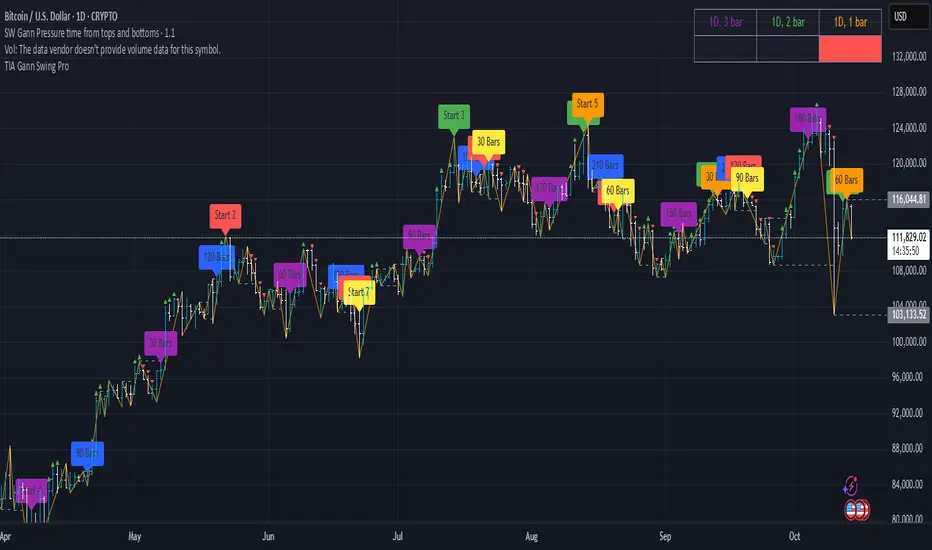
SW Gann Pressure time from tops and bottomsW.D. Gann's trading techniques often emphasized the significance of time in the markets, believing that specific time intervals could influence price movements. Here’s how the 30, 60, 90, 120, 180, and 270 bar intervals relate to Gann's rules:
1. **30 Bars**:
- Gann often viewed shorter time frames as critical for identifying short-term trends. A 30-bar interval can signify minor cycles or potential turning points in price.
2. **60 Bars**:
- This interval is significant as Gann believed in the importance of quarterly cycles. A 60-bar mark could indicate a completion of a two-month cycle, often leading to retracements or reversals.
3. **90 Bars**:
- Gann considered 90 days (or bars) to represent a quarter. This interval can signify a substantial shift in market sentiment or a pivotal point in a longer trend.
4. **120 Bars**:
- The 120-bar mark corresponds to about four months. Gann viewed longer intervals as more significant, often leading to major shifts in market trends.
5. **180 Bars**:
- A 180-bar period relates to a semi-annual cycle, which Gann regarded as critical for major support and resistance levels. Price action around this interval can reveal potential long-term trend reversals.
6. **270 Bars**:
- Gann believed that longer cycles, such as 270 bars (approximately nine months), could indicate significant market phases. This interval may represent major turning points and help identify long-term trends.
### Application in Trading:
- **Identifying Trends**: Traders can use these intervals to spot potential trend reversals or continuations based on Gann’s principles of market cycles.
- **Setting Targets and Stops**: Knowing where these key bars fall can help in setting profit targets and stop-loss orders.
- **Analyzing Market Sentiment**: Price reactions at these intervals can provide insights into market psychology and sentiment shifts.
By marking these intervals on a chart, traders can visually assess when price action aligns with Gann's theories, helping them make more informed trading decisions based on historical patterns and cycles.
Overnight Positioning w EMA - Strategy [presentTrading]I've recently started researching Market Timing strategies, and it’s proving to be quite an interesting area of study. The idea of predicting optimal times to enter and exit the market, based on historical data and various indicators, brings a dynamic edge to trading. Additionally, it is integrated with the 3commas bot for automated trade execution.
I'm still working on it. Welcome to share your point of view.
█ Introduction and How it is Different
The "Overnight Positioning with EMA " is designed to capitalize on market inefficiencies during the overnight trading period. This strategy takes a position shortly before the market closes and exits shortly after it opens the following day. What sets this strategy apart is the integration of an optional Exponential Moving Average (EMA) filter, which ensures that trades are aligned with the underlying trend. The strategy provides flexibility by allowing users to select between different global market sessions, such as the US, Asia, and Europe.
It is integrated with the 3commas bot for automated trade execution and has a built-in mechanism to avoid holding positions over the weekend by force-closing positions on Fridays before the market closes.
BTCUSD 20 mins Performance
█ Strategy, How it Works: Detailed Explanation
The core logic of this strategy is simple: enter trades before market close and exit them after market open, taking advantage of potential price movements during the overnight period. Here’s how it works in more detail:
🔶 Market Timing
The strategy determines the local market open and close times based on the selected market (US, Asia, Europe) and adjusts entry and exit points accordingly. The entry is triggered a specific number of minutes before market close, and the exit is triggered a specific number of minutes after market open.
🔶 EMA Filter
The strategy includes an optional EMA filter to help ensure that trades are taken in the direction of the prevailing trend. The EMA is calculated over a user-defined timeframe and length. The entry is only allowed if the closing price is above the EMA (for long positions), which helps to filter out trades that might go against the trend.
The EMA formula:
```
EMA(t) = +
```
Where:
- EMA(t) is the current EMA value
- Close(t) is the current closing price
- n is the length of the EMA
- EMA(t-1) is the previous period's EMA value
🔶 Entry Logic
The strategy monitors the market time in the selected timezone. Once the current time reaches the defined entry period (e.g., 20 minutes before market close), and the EMA condition is satisfied, a long position is entered.
- Entry time calculation:
```
entryTime = marketCloseTime - entryMinutesBeforeClose * 60 * 1000
```
🔶 Exit Logic
Exits are triggered based on a specified time after the market opens. The strategy checks if the current time is within the defined exit period (e.g., 20 minutes after market open) and closes any open long positions.
- Exit time calculation:
exitTime = marketOpenTime + exitMinutesAfterOpen * 60 * 1000
🔶 Force Close on Fridays
To avoid the risk of holding positions over the weekend, the strategy force-closes any open positions 5 minutes before the market close on Fridays.
- Force close logic:
isFriday = (dayofweek(currentTime, marketTimezone) == dayofweek.friday)
█ Trade Direction
This strategy is designed exclusively for long trades. It enters a long position before market close and exits the position after market open. There is no shorting involved in this strategy, and it focuses on capturing upward momentum during the overnight session.
█ Usage
This strategy is suitable for traders who want to take advantage of price movements that occur during the overnight period without holding positions for extended periods. It automates entry and exit times, ensuring that trades are placed at the appropriate times based on the market session selected by the user. The 3commas bot integration also allows for automated execution, making it ideal for traders who wish to set it and forget it. The strategy is flexible enough to work across various global markets, depending on the trader's preference.
█ Default Settings
1. entryMinutesBeforeClose (Default = 20 minutes):
This setting determines how many minutes before the market close the strategy will enter a long position. A shorter duration could mean missing out on potential movements, while a longer duration could expose the position to greater price fluctuations before the market closes.
2. exitMinutesAfterOpen (Default = 20 minutes):
This setting controls how many minutes after the market opens the position will be exited. A shorter exit time minimizes exposure to market volatility at the open, while a longer exit time could capture more of the overnight price movement.
3. emaLength (Default = 100):
The length of the EMA affects how the strategy filters trades. A shorter EMA (e.g., 50) reacts more quickly to price changes, allowing more frequent entries, while a longer EMA (e.g., 200) smooths out price action and only allows entries when there is a stronger underlying trend.
The effect of using a longer EMA (e.g., 200) would be:
```
EMA(t) = +
```
4. emaTimeframe (Default = 240):
This is the timeframe used for calculating the EMA. A higher timeframe (e.g., 360) would base entries on longer-term trends, while a shorter timeframe (e.g., 60) would respond more quickly to price movements, potentially allowing more frequent trades.
5. useEMA (Default = true):
This toggle enables or disables the EMA filter. When enabled, trades are only taken when the price is above the EMA. Disabling the EMA allows the strategy to enter trades without any trend validation, which could increase the number of trades but also increase risk.
6. Market Selection (Default = US):
This setting determines which global market's open and close times the strategy will use. The selection of the market affects the timing of entries and exits and should be chosen based on the user's preference or geographic focus.

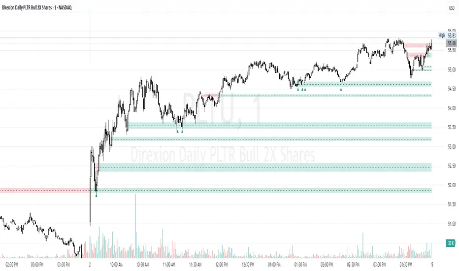
Control Candle Range [UkutaLabs]Control Candle Range
█ OVERVIEW
The Control Candle Range is a powerful trading tool that automatically identifies control candles in real time. The versatile ranges drawn by this indicator can be used in a variety of trading strategies because they can be used as ranges as well as areas of support and resistance.
The purpose of this script is to simplify the trading experience of users by automatically identifying and displaying Control Candle Ranges.
█ USAGE
A Control Candle is a candle that is followed by two consecutive inside candles. When this pattern is detected, this indicator will automatically identify it and draw a range in real time. This range will continue to extend as long as candles continue to close within the range of the Control Candle. It is important to note that a Control Candle is still valid if the price action exits its range as long as it closes within its range.
This script also supports higher time frame mapping, allowing you to draw Control Candle Ranges from higher timeframes onto lower timeframe charts. This is a powerful feature that allows users to see multiple timeframes worth of information at a glance on one single chart.
Each Control Candle Range will also be displayed with a label to allow users to understand at a glance which timeframe the range is being drawn from. These labels can be turned off in the settings.
The user also has the ability to adjust the color of each timeframe’s ranges.
█ SETTINGS
Configuration
• Show Labels: Determines whether or not identifying labels are displayed on ranges.
• Label Size: Determines the size of labels.
• Text Alignment: Determines where labels are drawn on ranges.
• Max Display: Determines the maximum number of ranges that can be drawn from each timeframe.
Current Timeframe
• Display (On/Off): Determines whether or not ranges from the current timeframe will be drawn on the chart.
• Color: Determines the color of ranges drawn from the current timeframe.
5 Minute (Higher Timeframe)
• Display (On/Off): Determines whether or not ranges from the 5 minute timeframe will be drawn on the chart.
• Color: Determines the color of ranges drawn from the 5 minute timeframe.
15 Minute (Higher Timeframe)
• Display (On/Off): Determines whether or not ranges from the 15 minute timeframe will be drawn on the chart.
• Color: Determines the color of ranges drawn from the 15 minute timeframe.
30 Minute (Higher Timeframe)
• Display (On/Off): Determines whether or not ranges from the 30 minute timeframe will be drawn on the chart.
• Color: Determines the color of ranges drawn from the 30 minute timeframe.
60 Minute (Higher Timeframe)
• Display (On/Off): Determines whether or not ranges from the 60 minute timeframe will be drawn on the chart.
• Color: Determines the color of ranges drawn from the 60 minute timeframe.
240 Minute (Higher Timeframe)
• Display (On/Off): Determines whether or not ranges from the 240 minute timeframe will be drawn on the chart.
• Color: Determines the color of ranges drawn from the 240 minute timeframe.
Daily (Higher Timeframe)
• Display (On/Off): Determines whether or not ranges from the daily timeframe will be drawn on the chart.
• Color: Determines the color of ranges drawn from the daily timeframe.

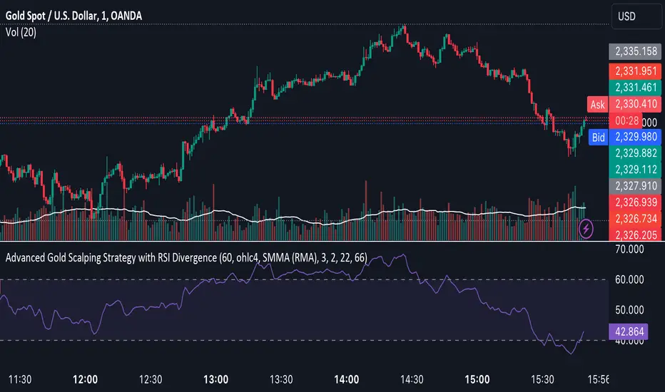
Advanced Gold Scalping Strategy with RSI Divergence# Advanced Gold Scalping Strategy with RSI Divergence
## Overview
This Pine Script implements an advanced scalping strategy for gold (XAUUSD) trading, primarily designed for the 1-minute timeframe. The strategy utilizes the Relative Strength Index (RSI) indicator along with its moving average to identify potential trade setups based on divergences between price action and RSI movements.
## Key Components
### 1. RSI Calculation
- Uses a customizable RSI length (default: 60)
- Allows selection of the source for RSI calculation (default: close price)
### 2. Moving Average of RSI
- Supports multiple MA types: SMA, EMA, SMMA (RMA), WMA, VWMA, and Bollinger Bands
- Customizable MA length (default: 3)
- Option to display Bollinger Bands with adjustable standard deviation multiplier
### 3. Divergence Detection
- Implements both bullish and bearish divergence identification
- Uses pivot high and pivot low points to detect divergences
- Allows for customization of lookback periods and range for divergence detection
### 4. Entry Conditions
- Long Entry: Bullish divergence when RSI is below 40
- Short Entry: Bearish divergence when RSI is above 60
### 5. Trade Management
- Stop Loss: Customizable, default set to 11 pips
- Take Profit: Customizable, default set to 33 pips
### 6. Visualization
- Plots RSI line and its moving average
- Displays horizontal lines at 30, 50, and 70 RSI levels
- Shows Bollinger Bands when selected
- Highlights divergences with "Bull" and "Bear" labels on the chart
## Input Parameters
- RSI Length: Adjusts the period for RSI calculation
- RSI Source: Selects the price source for RSI (close, open, high, low, hl2, hlc3, ohlc4)
- MA Type: Chooses the type of moving average applied to RSI
- MA Length: Sets the period for the moving average
- BB StdDev: Adjusts the standard deviation multiplier for Bollinger Bands
- Show Divergence: Toggles the display of divergence labels
- Stop Loss: Sets the stop loss distance in pips
- Take Profit: Sets the take profit distance in pips
## Strategy Logic
1. **RSI Calculation**:
- Computes RSI using the specified length and source
- Calculates the chosen type of moving average on the RSI
2. **Divergence Detection**:
- Identifies pivot points in both price and RSI
- Checks for higher lows in RSI with lower lows in price (bullish divergence)
- Checks for lower highs in RSI with higher highs in price (bearish divergence)
3. **Trade Entry**:
- Enters a long position when a bullish divergence is detected and RSI is below 40
- Enters a short position when a bearish divergence is detected and RSI is above 60
4. **Position Management**:
- Places a stop loss order at the entry price ± stop loss pips (depending on the direction)
- Sets a take profit order at the entry price ± take profit pips (depending on the direction)
5. **Visualization**:
- Plots the RSI and its moving average
- Draws horizontal lines for overbought/oversold levels
- Displays Bollinger Bands if selected
- Shows divergence labels on the chart for identified setups
## Usage Instructions
1. Apply the script to a 1-minute XAUUSD (Gold) chart in TradingView
2. Adjust the input parameters as needed:
- Increase RSI Length for less frequent but potentially more reliable signals
- Modify MA Type and Length to change the sensitivity of the RSI moving average
- Adjust Stop Loss and Take Profit levels based on current market volatility
3. Monitor the chart for Bull (long) and Bear (short) labels indicating potential trade setups
4. Use in conjunction with other analysis and risk management techniques
## Considerations
- This strategy is designed for short-term scalping and may not be suitable for all market conditions
- Always backtest and forward test the strategy before using it with real capital
- The effectiveness of divergence-based strategies can vary depending on market trends and volatility
- Consider using additional confirmation signals or filters to improve the strategy's performance
Remember to adapt the strategy parameters to your risk tolerance and trading style, and always practice proper risk management.
ICT IPDA Liquidity Matrix By AlgoCadosThe ICT IPDA Liquidity Matrix by AlgoCados is a sophisticated trading tool that integrates the principles of the Interbank Price Delivery Algorithm (IPDA), as taught by The Inner Circle Trader (ICT). This indicator is meticulously designed to support traders in identifying key institutional levels and liquidity zones, enhancing their trading strategies with data-driven insights. Suitable for both day traders and swing traders, the tool is optimized for high-frequency and positional trading, providing a robust framework for analyzing market dynamics across multiple time horizons.
# Key Features
Multi-Time Frame Analysis
High Time Frame (HTF) Levels : The indicator tracks critical trading levels over multiple days, specifically at 20, 40, and 60-day intervals. This functionality is essential for identifying long-term trends and significant support and resistance levels that aid in strategic decision-making for swing traders and positional traders.
Low Time Frame (LTF) Levels : It monitors price movements within 20, 40, and 60-hour intervals on lower time frames. This granularity provides a detailed view of intraday price actions, which is crucial for scalping and short-term trading strategies favored by day traders.
Daily Open Integration : The indicator includes the daily opening price, providing a crucial reference point that reflects the market's initial sentiment. This feature helps traders assess the market's direction and volatility, enabling them to make informed decisions based on the day's early movements, which is particularly useful for day trading strategies.
IPDA Reference Points : By leveraging IPDA's 20, 40, and 60-period lookbacks, the tool identifies Key Highs and Lows, which are used by IPDA as Draw On Liquidity. IPDA is an electronic and algorithmic system engineered for achieving price delivery efficiency, as taught by ICT. These reference points serve as benchmarks for understanding institutional trading behavior, allowing traders to align their strategies with the dominant market forces and recognize institutional key levels.
Dynamic Updates and Overlap Management : The indicator is updated daily at the beginning of a new daily candle with the latest market data, ensuring that traders operate with the most current information. It also features intelligent overlap management that prioritizes the most relevant levels based on the timeframe hierarchy, reducing visual clutter and enhancing chart readability.
Comprehensive Customization Options : Traders can tailor the indicator to their specific needs through an extensive input menu. This includes toggles for visibility, line styles, color selections, and label display preferences. These customization options ensure that the tool can adapt to various trading styles and preferences, enhancing user experience and analytical capabilities.
User-Friendly Interface : The tool is designed with a user-friendly interface that includes clear, concise labels for all significant levels. It supports various font families and sizes, making it easier to interpret and act upon the displayed data, ensuring that traders can focus on making informed trading decisions without being overwhelmed by unnecessary information.
# Usage Note
The indicator is segmented into two key functionalities:
LTF Displays : The Low Time Frame (LTF) settings are exclusive to timeframes up to 1 hour, providing detailed analysis for intraday traders. This is crucial for traders who need precise and timely data to make quick decisions within the trading day.
HTF Displays : The High Time Frame (HTF) settings apply to the daily timeframe and any shorter intervals, allowing for comprehensive analysis over extended periods. This is beneficial for swing traders looking to identify broader trends and market directions.
# Inputs and Configurations
BINANCE:BTCUSDT
Offset: Adjustable setting to shift displayed data horizontally for better visibility, allowing traders to view past levels and make informed decisions based on historical data.
Label Styles: Choose between compact or verbose label formats for different levels, offering flexibility in how much detail is displayed on the chart.
Daily Open Line: Customizable line style and color for the daily opening price, providing a clear visual reference for the start of the trading day.
HTF Levels: Configurable high and low lines for HTF with options for style and color customization, allowing traders to highlight significant levels in a way that suits their trading style.
LTF Levels: Similar customization options for LTF levels, ensuring flexibility in how data is presented, making it easier for traders to focus on the most relevant intraday levels.
Text Utils: Settings for font family, size, and text color, allowing for personalized display preferences and ensuring that the chart is both informative and aesthetically pleasing.
# Advanced Features
Overlap Management : The script intelligently handles overlapping levels, particularly where multiple timeframes intersect, by prioritizing the more significant levels and removing redundant ones. This ensures that the charts remain clear and focused on the most critical data points, allowing traders to concentrate on the most relevant market information.
Real-Time Updates : The indicator updates its calculations at the start of each new daily bar, incorporating the latest market data to provide timely and accurate trading signals. This real-time updating is crucial for traders who rely on up-to-date information to execute their strategies effectively and make informed trading decisions.
# Example Use Cases
Scalpers/Day traders: Can utilize the LTF features to make rapid decisions based on hourly market movements, identifying short-term trading opportunities with precision.
Swing Traders: Will benefit from the HTF analysis to identify broader trends and key levels that influence longer-term market movements, enabling them to capture significant market swings.
By providing a clear, detailed view of key market dynamics, the ICT IPDA Liquidity Matrix by AlgoCados empowers traders to make more informed and effective trading decisions, aligning with institutional trading methodologies and enhancing their market understanding.
# Usage Disclaimer
This tool is designed to assist in trading decisions, but it should be used in conjunction with other analysis methods and risk management strategies. Trading involves significant risk, and it is essential to understand the market conditions thoroughly before making trading decisions.

BINANCE-BYBIT Cross Chart: Spot-Perpetual CorrelationName: "Binance-Bybit Cross Chart: Spot-Perpetual Correlation"
Category: Scalping, Trend Analysis
Timeframe: 1M, 5M, 30M, 1D (depending on the specific technique)
Technical analysis: This indicator facilitates a comparison between the price movements shown on the Binance spot chart and the Bybit perpetual chart, with the aim of discerning the correlation between the two charts and identifying the dominant market trends. It automatically generates the corresponding chart based on the ticker selected in the primary chart. When a Binance pair is selected in the main chart, the indicator replicates the Bybit perpetual chart for the same pair and timeframe, and vice versa, selecting the Bybit perpetual chart as the primary chart generates the Binance spot chart.
Suggested use: You can utilize this tool to conduct altcoin trading on Binance or Bybit, facilitating the comparison of price actions and real-time monitoring of trigger point sensitivity across both exchanges. We recommend prioritizing the Binance Spot chart in the main panel due to its typically longer historical data availability compared to Bybit.
The primary objective is to efficiently and automatically manage the following three aspects:
- Data history analysis for higher timeframes, leveraging the extensive historical data of the Binance spot market. Variations in indicators such as slow moving averages may arise due to differences in historical data between exchanges.
- Assessment of coin liquidity on both exchanges by observing candlestick consistency on smaller timeframes or the absence of gaps. In the crypto market, clean charts devoid of gaps indicate dominance and offer enhanced reliability.
- Identification of precise trigger point levels, including daily, previous day, or previous week highs and lows, which serve as sensitive areas for breakout or reversal operations.
All-Time High (ATH) and All-Time Low (ATL) levels may vary significantly across exchanges due to disparities in historical data series.
This tool empowers traders to make informed decisions by leveraging historical data, liquidity insights, and precise trigger point identification across Binance Spot and Bybit Perpetual market.
Configuration:
EMA length:
- EMA 1: Default 5, user configurable
- EMA 2: Default 10, user configurable
- EMA 3: Default 60, user configurable
- EMA 4: Default 223, user configurable
- Additional Average: Optional display of an additional average, such as a 20-period average.
Chart Elements:
- Session separator: Indicates the beginning of the current session (in blue)
- Background: Indicates an uptrend (60 > 223) with a green background and a downtrend (60 < 223) with a red background.
Instruments:
- EMA Daily: Shows daily averages on an intraday timeframe.
- EMA levels 1h - 30m: Shows the levels of the 1g-30m EMAs.
- EMA Levels Highest TF: Provides the option to select additional EMA levels from the major timeframes, customizable via the drop-down menu.
- "Hammer Detector: Marks hammers with a green triangle and inverted hammers with a red triangle on the chart
- "Azzeramento" signal on TF > 30m: Indicates a small candlestick on the EMA after a dump.
- "No Fomo" signal on TF < 30m: Indicates a hyperextended movement.
Trigger Points:
- Today's highs and lows: Shows the opening price of the day's candlestick, along with the day's highs and lows (high in purple, low in red, open in green).
- Yesterday's highs and lows: Displays the opening price of the daily candlestick, along with the previous day's highs and lows (high in yellow, low in red).
You can customize the colors in "Settings" > "Style".
It is best used with the Scalping The Bull indicator on the main panel.
Credits:
@tumiza999: for tests and suggestions.
Thanks for your attention, happy to support the TradingView community.

AWR_WaveTrend Multitimeframe [adapted from LazyBear]I've adapted a script from Lazy Bear (WT trend oscillator)
WaveTrend Oscillator is a port of a famous TS/MT indicator.
When the oscillator (WT1 designed as a line) is above the overbought band (50 to 60) and crosses down the WT2 (dotted line), it is usually a good SELL signal. Similarly, when the oscillator crosses above the signal when below the Oversold band ( (-50 to -60)), it is a good BUY signal.
In this indicator, you can display at the same time, different time frames.
Choice possible are 1 mn, 15 mn, 30 mn, 60 mn, 120 mn, 240 mn, 1D, Week, Month.
Small time frames (1 to 30 mn) are represented by a blue lines (light to dark)
1H is in grey
2H & 4H are in purple (light to dark)
1D is in green
1W is in orange
1M is in black
You can choose which timeframes you want to display for the current period or for the last period closed.
In a few seconds, you perfectly see the selected timeframes trends.
There is also at the bottom right a table summing up all the different values of WT1, WT2 and difference between them.
Positive difference means an upside trend
Negative difference means a downside trend.
Another way of using this indicator is displaying only the difference between WT1 & WT2. It's giving the speed & the direction of all trends. Trends are our friends ...
You can observe the significent times frames and look if they are all positives or negatives or if the speed of lower timeframe cross a longer timeframe of if the speed is decreasing or increasing...
Difference values goes generaly from -20 to 20 (it can exceed a bit but really rare). 12 is already high level of speed.
Many uses possible.
In the exemple posted, I've selected WT1 and WT2 for timeframes 4H, Daily & Weekly.
Marker 1:
Orange lines (WT1) are far below - 50 (-67 here) and cross WT2 pointed lines : weekly buy signal
But this buy signal is balanced by 4H & Daily sell signal = it's marking start of hesitations of main trend !!!!
Marker 2 :
Next buy signal in 4H or daily would normaly confirm the start
Marker 3 :
Sell signal in 4H and daily but weekly has an upside trend ! Start of a counter trend in the trend. To find the perfect timing of that you have to look to lower time frames, because 4H and daily are giving many hesitations signals crossing down & crossing up many times in an overbought zone.
Marker 4 :
End of the counter trend. Most of the time, the countertrend don't go in the "over" zone. That's why if you trading in an counter trend, you have to keep it in mind.
Then a few days later you can see the sell signal. And what a sell signal ! 4H & daily are smashed down really fastly ! Trends change warning !
Marker 5
Long hesitation/change of the trend. Daily WT and 4H are below the weekly trends. Weekly start to go down.
Start of a counter trend inside the trend giving us the best selling signal at her end !
Marker 6 :
Long hesitation/change of the trend.
You have to look in lower time frames to identify the short trend. Difficult to find the best timing to get in. ....
I've add many alerts. When a time frame become positive or negative. When many time frames are positive or negative or above or below 47 level...
Please feel free to explore.
Hope it will help you.
Thanks to Lazybear ! Thousands thanks to Lazybear !
Exemple with difference

Rate of Change RSIIndicator Name: Rate of Change RSI
Description:
The Rate of Change (ROC) of the Relative Strength Index (RSI) is a technical indicator designed to provide insights into the momentum of an asset's price movement. It combines the Relative Strength Index (RSI), a popular momentum oscillator, with the Rate of Change (ROC) concept to assess the speed at which RSI values are changing.
How It Works:
Relative Strength Index (RSI): The RSI measures the magnitude of recent price changes to evaluate overbought or oversold conditions in an asset. It oscillates between 0 and 100, with readings above 70 typically indicating overbought conditions and readings below 30 indicating oversold conditions.
Rate of Change (ROC): The ROC calculates the percentage change in a given indicator over a specified period. In this indicator, we apply the ROC to the RSI values to determine how quickly the RSI is changing over time.
Key Features:
Acceleration and Deceleration: The ROC of RSI helps traders identify whether the momentum of the RSI is accelerating or decelerating. Positive values suggest increasing momentum, while negative values indicate decreasing momentum.
Dynamic Color Change: The color of the ROC RSI line changes dynamically based on the RSI level. When the RSI is between 0 and 40, the line color is blue, indicating potential oversold conditions. When the RSI is between 40 and 60, the line color is yellow, suggesting neutral conditions. When the RSI is above 60, the line color changes to green, indicating potential overbought conditions.
How to Use:
Acceleration: When the ROC RSI is positive and increasing while the RSI is above 60 (green), it may signal strong upward momentum.
Deceleration: Conversely, if the ROC RSI is negative and decreasing while the RSI is below 40 (blue), it may indicate weakening downward momentum.
Originality and Usefulness:
This indicator combines the RSI, a well-known momentum oscillator, with the ROC concept to provide a unique perspective on momentum dynamics. By dynamically adjusting the color of the ROC RSI line based on RSI levels, traders can quickly assess potential overbought or oversold conditions in the market.
Chart:
The chart displayed alongside this script provides a clean and easy-to-understand visualization of the ROC RSI indicator. The ROC RSI line color changes dynamically based on RSI levels, allowing traders to visually identify potential market conditions at a glance.

Trend Change IndicatorThe Trend Change Indicator is an all-in-one, user-friendly trend-following tool designed to identify bullish and bearish trends in asset prices. It features adjustable input values and a built-in alert system that promptly notifies investors of potential shifts in both short-term and long-term price trends. This alert system is crucial for helping less active investors correctly position themselves ahead of major trend shifts and assists in risk management after a trend is established. It's important to note that this indicator is most effective with assets that historically exhibit strong trends.
At the heart of this tool is the interaction between the 30-day and 60-day Exponential Moving Averages (EMA). A bullish trend is indicated in green when the 30-day EMA is above the 60-day EMA, while a bearish trend is signaled in red when the 30-day EMA is below the 60-day EMA. The appearance of gray alerts users to potential shifts in the current trend as the EMAs converge, falling below the Average True Range (ATR) safety margin. This analysis is conducted across both hourly and daily timeframes, with the 4-hour timeframe providing early signals for daily trend changes. The band visually represents the interaction between the daily EMAs and is also displayed in the second row of the table, with the first row showing the same EMA interaction on the 4-hour timeframe.
This indicator also includes a 140-day (20-week) Simple Moving Average (SMA), visually represented by a line with predictive dots. This feature significantly enhances the investor's ability to understand long-term trends in asset prices, offering forward-looking insights by projecting the SMA value 10 days into the future. The value of this forecast lies in interpreting the slope of the dots; upward trending dots suggest a bullish underlying trend, while downward trending dots indicate a bearish trend. Generally, prices above the SMA signal bullishness, and prices below indicate bearishness.
In summary, the Trend Change Indicator is a comprehensive solution for identifying price trends and managing risk. Its intuitive, color-coded design makes it an indispensable tool for traders and investors who aim to be well-positioned ahead of trend shifts and manage risk once a trend has been established. While it has proven historically valuable in trending markets such as cryptocurrencies, tech stocks, and commodities, it is advisable to use this indicator in conjunction with other technical analysis tools for a more comprehensive and well-rounded decision-making process.

RSI & Backed-Weighted MA StrategyRSI & MA Strategy :
INTRODUCTION :
This strategy is based on two well-known indicators that work best together: the Relative Strength Index (RSI) and the Moving Average (MA). We're going to use the RSI as a trend-follower indicator, rather than a reversal indicator as most are used to. To the signals sent by the RSI, we'll add a condition on the chart's MA, filtering out irrelevant signals and considerably increasing our winning rate. This is a medium/long-term strategy. There's also a money management method enabling us to reinvest part of the profits or reduce the size of orders in the event of substantial losses.
RSI :
The RSI is one of the best-known and most widely used indicators in trading. Its purpose is to warn traders when an asset is overbought or oversold. It was designed to send reversal signals, but we're going to use it as a trend indicator by increasing its length to 20. The RSI formula is as follows :
RSI (n) = 100 - (100 / (1 + (H (n)/L (n))))
With n the length of the RSI, H(n) the average of days closing above the open and L(n) the average of days closing below the open.
MA :
The Moving Average is also widely used in technical analysis, to smooth out variations in an asset. The SMA formula is as follows :
SMA (n) = (P1 + P2 + ... + Pn) / n
where n is the length of the MA.
However, an SMA does not weight any of its terms, which means that the price 10 days ago has the same importance as the price 2 days ago or today's price... That's why in this strategy we use a RWMA, i.e. a back-weighted moving average. It weights old prices more heavily than new ones. This will enable us to limit the impact of short-term variations and focus on the trend that was dominating. The RWMA used weights :
The 4 most recent terms by : 100 / (4+(n-4)*1.30)
The other oldest terms by : weight_4_first_term*1.30
So the older terms are weighted 1.30 more than the more recent ones. The moving average thus traces a trend that accentuates past values and limits the noise of short-term variations.
PARAMETERS :
RSI Length : Lenght of RSI. Default is 20.
MA Type : Choice between a SMA or a RWMA which permits to minimize the impact of short term reversal. Default is RWMA.
MA Length : Length of the selected MA. Default is 19.
RSI Long Signal : Minimum value of RSI to send a LONG signal. Default is 60.
RSI Short signal : Maximum value of RSI to send a SHORT signal. Default is 40.
ROC MA Long Signal : Maximum value of Rate of Change MA to send a LONG signal. Default is 0.
ROC MA Short signal : Minimum value of Rate of Change MA to send a SHORT signal. Default is 0.
TP activation in multiple of ATR : Threshold value to trigger trailing stop Take Profit. This threshold is calculated as multiple of the ATR (Average True Range). Default value is 5 meaning that to trigger the trailing TP the price need to move 5*ATR in the right direction.
Trailing TP in percentage : Percentage value of trailing Take Profit. This Trailing TP follows the profit if it increases, remaining selected percentage below it, but stops if the profit decreases. Default is 3%.
Fixed Ratio : This is the amount of gain or loss at which the order quantity is changed. Default is 400, which means that for each $400 gain or loss, the order size is increased or decreased by a user-selected amount.
Increasing Order Amount : This is the amount to be added to or subtracted from orders when the fixed ratio is reached. The default is $200, which means that for every $400 gain, $200 is reinvested in the strategy. On the other hand, for every $400 loss, the order size is reduced by $200.
Initial capital : $1000
Fees : Interactive Broker fees apply to this strategy. They are set at 0.18% of the trade value.
Slippage : 3 ticks or $0.03 per trade. Corresponds to the latency time between the moment the signal is received and the moment the order is executed by the broker.
Important : A bot has been used to test the different parameters and determine which ones maximize return while limiting drawdown. This strategy is the most optimal on BITSTAMP:ETHUSD with a timeframe set to 6h. Parameters are set as follows :
MA type: RWMA
MA Length: 19
RSI Long Signal: >60
RSI Short Signal : <40
ROC MA Long Signal : <0
ROC MA Short Signal : >0
TP Activation in multiple ATR : 5
Trailing TP in percentage : 3
ENTER RULES :
The principle is very simple:
If the asset is overbought after a bear market, we are LONG.
If the asset is oversold after a bull market, we are SHORT.
We have defined a bear market as follows : Rate of Change (20) RWMA < 0
We have defined a bull market as follows : Rate of Change (20) RWMA > 0
The Rate of Change is calculated using this formula : (RWMA/RWMA(20) - 1)*100
Overbought is defined as follows : RSI > 60
Oversold is defined as follows : RSI < 40
LONG CONDITION :
RSI > 60 and (RWMA/RWMA(20) - 1)*100 < -1
SHORT CONDITION :
RSI < 40 and (RWMA/RWMA(20) - 1)*100 > 1
EXIT RULES FOR WINNING TRADE :
We have a trailing TP allowing us to exit once the price has reached the "TP Activation in multiple ATR" parameter, i.e. 5*ATR by default in the profit direction. TP trailing is triggered at this point, not limiting our gains, and securing our profits at 3% below this trigger threshold.
Remember that the True Range is : maximum(H-L, H-C(1), C-L(1))
with C : Close, H : High, L : Low
The Average True Range is therefore the average of these TRs over a length defined by default in the strategy, i.e. 20.
RISK MANAGEMENT :
This strategy may incur losses. The method for limiting losses is to set a Stop Loss equal to 3*ATR. This means that if the price moves against our position and reaches three times the ATR, we exit with a loss.
Sometimes the ATR can result in a SL set below 10% of the trade value, which is not acceptable. In this case, we set the SL at 10%, limiting losses to a maximum of 10%.
MONEY MANAGEMENT :
The fixed ratio method was used to manage our gains and losses. For each gain of an amount equal to the value of the fixed ratio, we increase the order size by a value defined by the user in the "Increasing order amount" parameter. Similarly, each time we lose an amount equal to the value of the fixed ratio, we decrease the order size by the same user-defined value. This strategy increases both performance and drawdown.
Enjoy the strategy and don't forget to take the trade :)
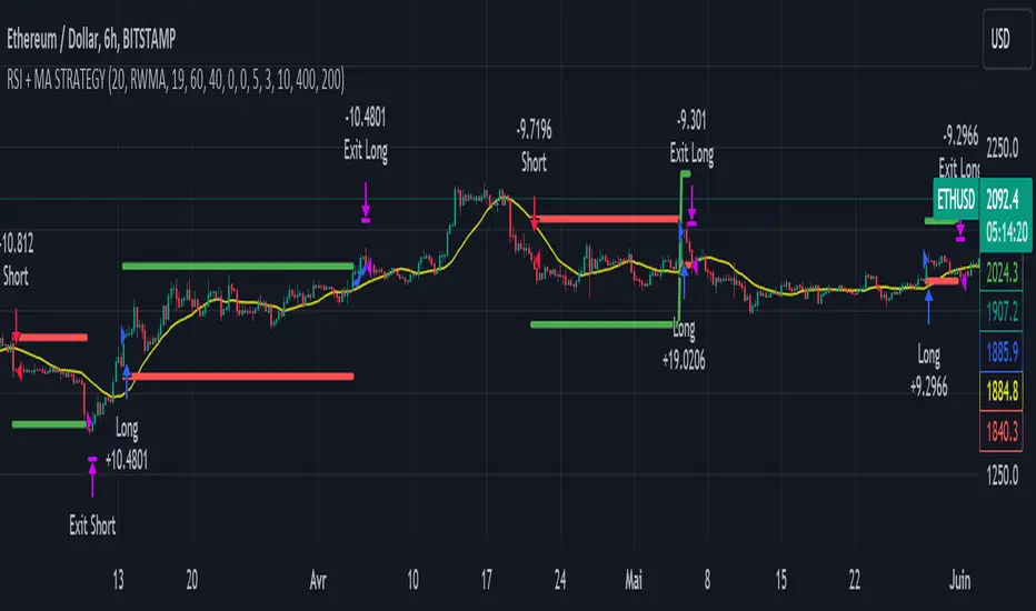
RSI + Fibonacci HH LL Support Resistance I have integrated my past scripts and brushed them up further.
This tool allows for support/resistance, stop loss, take profit, and trend analysis using RSI and Fibonacci ratios.
For example, the Fibonacci ratio is used as follows
l1 = m - dist * 0.618
l2 = m - dist * 1.618
l3 = m - dist * 2.618
l4 = m - dist * 4.235
l5 = m - dist * 6.857
l6 = m - dist * 11.089
When the Fibonacci ratio reaches 2.618 or higher and the RSI smoothed by the 5-day EMA is oversold/overbought, the bar color is changed by a gradation.
We have tried to make the design as beautiful and good-looking as possible. You can also hide the lines to suit your own preference.
Example usages are here:
BTCUSDT 1Hour Chart
Using Fibonacci numbers
BTCUSDT 15min Chart, for Scalping
Here, to set the highest and lowest prices one hour ago, "4" is substituted as the calculation: 15 minutes x 4 = 60
BTCUSDT 15min Chart, for Scalping
To set the highest and lowest prices 4 hours ago , "4" is substituted as the calculation: 15 minutes x 16 = 240
BTCUSDT 15min Chart, for Scalping
To draw yesterday's high and low as support/resistance lines, I substituted the number "96" as 1440/15=96.
BTCUSDT 1min Chart, for Scalping
Substituted "60" to trail the highest and lowest prices over a 60-minute period on a 1-minute chart, and removed lines to beautify
BTCUSDT 1day Chart, for Long-Term Investers
This is an example of using "90" because it is a 1-day chart and assumes that 3 months = 90 days in order to trail the highest and lowest prices over a 3-month period and no lines.
My past scripts are here:
RSI + FIB HH LL StopLoss Finder/Contrarian Trades
Fibonacci HH LL TRAMA Band

Machine Learning: MFI Heat Map [YinYangAlgorithms]Overview:
MFI Heat Maps are a visually appealing way to display the values of 29 different MFIs at the same time while being able to make sense of it. Each plot within the Indicator represents a different MFI value. The higher you get up, the longer the length that was used for this MFI. This Indicator also features the use of Machine Learning to help balance the MFI levels. It doesn’t solely rely upon Machine Learning but instead incorporates a growing length MFI averaged with the Machine Learning MFI at any given index.
For instance, say we are calculating the 10th plot from the bottom, the MFI would be an average of:
MFI(source, 11)
Machine Learning MFI at Index of 10
We do it this way as they both help smooth each other out without relying solely on just one calculation method.
Due to plot limitations, you are capped at 28 Plot Amounts within this indicator, but that is still quite a bit of information you can glean from a Heat Map.
The Machine Learning used in this indicator is of the K-Nearest Neighbor (KNN). It uses a Fast and Slow MFI calculation then sorts through them over Machine Learning Length and calculates the differences between them. It then slices off KNN length to create our Max/Min Distances allotted. It adds the average between Fast and Slow MFIs to a Viable Distances array if their distances are within the KNN Min/Max distance. It then averages all distances in the Viable Distances array and returns the result.
The result of the KNN Function is saved to another ML Data array whose length is that of Plot Amount (Heat Map Size). This way each Index of the ML Data array can be indexed according to the Heat Map Size.
The Average of the ML Data array is the MFI line (white) that you’ll see plotted on the Indicator. There is also the SMA of the MFI Average (orange) which is likewise plotted. These plots allow you to visualize where the ML MFI is sitting and can potentially be useful for seeing when the MFI Average and SMA cross over and under each other.
We’ve heard many people talk highly of RSI, but sadly not too many even refer to MFI. MFI oftentimes may be overlooked, especially with new traders who may not even know what it is. Essentially MFI is an RSI but it also incorporates Volume into its calculations, which in our opinion leads to a more accurate reading; afterall, what is price movement without Volume.
Tutorial:
You may be thinking, this Indicator looks appealing to the eye, but how do I benefit from it trading wise?
Before we get into our visual examples, let's talk briefly about what makes Heat Maps in general a useful tool for trading. Heat Maps give us the ability to visualize and understand lots of data while removing the clutter. We can understand the data of 29 different MFIs without having to look at and decipher 29 different MFI plots. When you overlay too many MFI lines on top of each other, they can be very difficult to read and oftentimes end up actually hindering your Technical Analysis. For this reason, we have a simple solution to this problem; Heat Maps. This MFI Heat Map allows you to easily know (in a relative %) what the MFI level is for varying lengths. For Instance, the First (bottom) plot indexes an MFI of (K(0) (loop of Plot Amount) + Smoothing Length (default 1)) = 1. Since this is indexing (usually) a very low length, it will change much quicker. Whereas the Last (top) plot indexes an MFI of (K(27) (loop of Plot Amount) + Smoothing Length (default 1)) = 28. This is indexing a much higher length of MFI which results in the MFI the higher you go up in the Heat Map to move much slower.
Heat Maps give us the ability to see changes happening over multiple MFIs at the same time, which can be very useful for seeing shifts in MFI / Momentum. Remember, MFI incorporates Volume, so even if the price goes up a lot, if there was low volume, the MFI won’t move as much as an RSI would. However, likewise, if there is high volume but low price movement, the MFI will move slightly more than the RSI.
Heat Maps change color based on their MFI level. If the MFI is >= 90 it is HOT (red), if the MFI <= 9 it is COLD (teal, think of ICE). Green represents an MFI of 50-59 and Dark Blue represents an MFI of 40-49. Green and Dark blue are the most common colors as all the others are more ‘Extreme’ MFI levels.
Okay, time to get to the Examples :
Since there is so much going on in Heat Maps, we’ve decided to focus this tutorial to this specific area and talk about individual locations before talking about it as a whole.
If you refer to the example above where there are 2 white circles; these white circles are highlighting a key location you’ll be wanting to identify within your Heat Maps, many things are happening here:
The MFI crossed over the SMA (bullish).
The Heat Map started changing from mid/dark Blue (30-50 MFI) to Green (50-59 MFI) around the midline (the 50% dashed like).
The Lower levels of the Heat Map are turning Yellow/Orange/Red (60-100 MFI).
The Upper Levels of the Heat Map are still Light Blue - Green (10-50 MFI).
The 4 Key points above, all point towards potential Bullish Momentum changes. You’re likely wondering, but why? Let's discuss about each one in more specific detail:
1. The MFI crossed over the SMA (bullish): What this tells us is that the current MFI Average is now greater than its average over the last (default) 16 bars. This means there's been a large amount of Money Flow (Price and Volume) recently (subjectively based on the last (default) 16 average). This is one of the leading Bullish / Bearish signals you will see within this Indicator. You can enable Signals within the Settings and/or even add Alerts for when these crossings occur.
2. The Heat Map started changing from mid/dark Blue (30-50 MFI) to Green (50-59 MFI) around the midline (the 50% dashed like): This shows us that the index’s in the mid (if using all 28 heat map plots it would be at 14) has already received some of this momentum change. If you look at the second white circle (right), you’ll also notice the higher MFI plot indexes are also green. This is because since their length is long they still have some momentum and strength from the first white circle (left). Just because the first white circle failed in its bullish push, doesn’t mean it didn’t achieve momentum that would later on help to push the price up.
3. The Lower levels of the Heat Map are turning Yellow/Orange/Red (60-100 MFI): It occurred somewhat in the left white circle, but mainly in the right white circle. This shows us the MFI is very high on the lower lengths, this may lead to the current, middle and higher length MFIs following suit soon. Remember it has to work its way up, the higher levels can’t go red unless the lower levels go red first and the higher levels can also lag quite a bit behind and take awhile to catch up, this is normal, expected and meant to happen. Vice versa is also true with getting higher levels to go cold (light teal (think of ICE)).
4. The Upper Levels of the Heat Map are still Light Blue - Green (10-50 MFI): You might think at first that this is a bad thing, but it's not! Remember you want to be Fearful when others are Greedy and Greedy when others are Fearful! You don’t want to buy when the higher levels have a high MFI, you want to buy when you see the momentum pushing up in the lower MFI levels (getting yellow/orange/red in the low levels) while it is still Cold in the higher levels (BLUE OR GREEN, nothing higher than green as it is already slightly too high). There will be many times that it is Yellow or possibly Orange in the high levels and the bullish push still happens, but this is much more risky! The key to trading is to minimize risks while maximizing potential.
Hopefully now you’re getting an idea of how to spot potential bullish momentum changes, but what about bearish momentum changes? Technically they are the exact opposite, so we don’t need to go into as much detail, but lets still take a look at a few examples:
In the example above we marked the 3 times where it was displaying overly bullish characteristics. We marked the bullish momentum occurring with arrows. If you look closely at the start of the arrow to where it finishes, you’ll notice how the heat (HOT)(RED) works its way up from the lower levels to the higher levels. We then see the MFI to SMA cross under. In all 3 of these examples the heat made it all the way to the top of the chart. These are all very bearish signals that represent a bearish momentum movement that may occur soon.
Also, please note, the level the MFI is at DOES matter! That line isn’t there simply for you to see when there are crosses over and under. The MFI is considered to be Overbought when it is greater than 70 (the upper white dashed line, it is just formatted to be on a different scale cause there are 28 plots, but it represents 70). The MFI is considered to be Oversold when it is less than 30 (the lower white dashed line).
If we look to the left a little here where a big drop in price occurred shortly after our MFI and SMA crossed, would we have been able to identify it using the Heat Maps? Likely, No. There was some color change in the lower levels a few bars prior that went yellow/orange/red but before this cross happened they all went back to Dark Blue. In the middle section when the cross happened it was only Green and Yellow and in the upper section we are Blue. This would be a very risky trade to go on as the only real Bearish Indication was the MFI to SMA cross under. Remember, you want to reduce risk, you don’t want to simply trade on everytime the MFI and SMA cross each other or you’ll be getting yourself into many risky trades based on false signals.
Based on what you’ve learned above, can you see the signs that are indicating where this white circle may have potential for a bullish momentum change?
Now that we are more zoomed in, you may also be noticing there are colors to the price bars. This can be disabled in the settings, but just so you know what they mean, let’s zoom in a little more and talk about it.
We’ve condensed the Indicator a bit so you can see the bars better here. The colors that are displayed on these bars are the Heat Map value for your MFI (the white line in the Indicator). This way you can better see when the Price is Hot and Cold. As you may see while looking, the colors generally go from cold to hot when bullish momentum is happening and hot to cold when bearish momentum is happening. We don’t recommend solely looking at the bars as indicators to MFI momentum change, as seeing the Heat Map will give you much more data; however it can be nice to see the Heat Map projected on the bars rather than trying to eyeball it yourself or hover over each bar specifically to see their levels.
We will conclude our Tutorial here. Hopefully this has given you some insight to how useful Heat Maps can be and why it works well with a Machine Learning (KNN) Model applied to the MFI.
PLEASE NOTE: You can adjust the line width for the Heat Map within the settings. If you condense the Indicator a lot or have a small screen, likely use a length of 1-2. If you have it stretched out or a large screen, a length of 2-3 will work nice. You just don’t want to have the lines overlapping or it defeats the purpose of a Heat Map. Also, the bigger the linewidth, generally you’ll want to increase the Transparency within the Settings also as it can get quite bright and hurt your eyes over time.
Settings:
MFI:
Show MFI and SMA Crossing Signals: MFI and SMA Crossing is one of the leading Bullish and Bearish Signals in this Indicator. You can also add alerts for these signals.
Plot Amount: How many plots are used in this Heat Map. (2 - 28).
Source: The Source to use in all MFI calculations.
Smooth Initial MFI Length: How much to smooth the Fast and Slow MFI calculation by. 1 = No smoothing.
MFI SMA Length: What length we smooth the MFI Average over to get our MFI SMA.
Machine Learning:
Average MFI data by adding a lookback to the Source: While populating our Heat Map with the MFI's, should use use the Source each MFI Length increase or should we also lookback a Source each MFI Length Increase.
KNN Distance Requirement: To be a valid KNN, it needs to abide by a Distance calculation. Generally only Max is used, but you can change it if it suits your trading style better.
Machine Learning Length: How much ML data should we store? The longer the length generally the smoother the result; which may not be as accurate for something like a Heat Map, so keeping this relatively low may lead to more accurate results.
KNN Length: How many KNN are used in the slice to calculate max/min distance allowed.
Fast Length: Fast MFI length used in KNN to calculate distances by comparing its distance with the Slow MFI Length.
Slow Length: Slow MFI length used in KNN to calculate distances by comparing its distance with the Fast MFI Length.
Smoothing Length: When populating our Heat Map, at what length do we start our MFI calculations with (A Higher value with result in a slower and more smoothed MFI / Heat Map).
Colors:
Change Bar Color: Change bar colors to MFI Avg Color.
Heat Map Transparency: If there isn't any transparency it can be a little hard on the eyes. The Greater the Line Width, generally the more transparency you'll want for your eyes.
Line Width: Set how wide the Heat Map lines are
MFI 90-100 Color: Color when the MFI is between these levels.
MFI 80-89 Color: Color when the MFI is between these levels.
MFI 70-79 Color: Color when the MFI is between these levels.
MFI 60-69 Color: Color when the MFI is between these levels.
MFI 50-59 Color: Color when the MFI is between these levels.
MFI 40-49 Color: Color when the MFI is between these levels.
MFI 30-39 Color: Color when the MFI is between these levels.
MFI 20-29 Color: Color when the MFI is between these levels.
MFI 10-19 Color: Color when the MFI is between these levels.
MFI 0-100 Color: Color when the MFI is between these levels.
If you have any questions, comments, ideas or concerns please don't hesitate to contact us.
HAPPY TRADING!

Initial Balance Panel Strategy for BitcoinInitial Balance Strategy
Initial Balance Strategy uses a source code of "Initial Balance Monitoring Panel" that build from "Initial Balance Markets Time Zones - Overall Highest and Lowest".
Initial Balance is based on the highest and lowest price action within the first 60 minutes of trading. Reading online this can depict which way the market can trend for the session. More information about Initial Balance Panel you can read at the end of the article.
Strategy idea
The main idea is to catch the trend move when most of the 16 Crypto pairs break the Low or High levels together. I found good results when 15 of 16 pairs is break that levels and after we manage the trade within some trail stop indicator, I choose Volatility Stop for this strategy.
Additional Strategy idea
The second one idea that was not made is to catch the pullback after fully green/red zones in Initial Balance Panel become white. That mean the main trend can be finished and we can try to catch good pullback in opposite direction.
Binance Crypto pairs
The strategy use the 16 default Crypto currencies pairs from the Binance. As additional variations of the strategy can be changing the currencies pairs and their number.
List of default pairs:
BINANCE:BTCUSDT, BINANCE:ETHUSDT, BINANCE:EOSUSDT, BINANCE:LTCUSDT, BINANCE:XRPUSDT, BINANCE:DASHUSDT, BINANCE:IOTAUSDT, BINANCE:NEOUSDT, BINANCE:QTUMUSDT, BINANCE:XMRUSDT, BINANCE:ZECUSDT, BINANCE:ETCUSDT, BINANCE:ADAUSDT, BINANCE:XTZUSDT, BINANCE:LINKUSDT, BINANCE:DOTUSDT
Summary
The strategy works very well for a buy trades with settings 15 crypto pairs of 16 that follow the trend with breaking the long initial balance level.
Initial Balance Monitoring Panel
Allows you to have an instant view of 16 Crypto pairs within a monitoring panel, monitoring Initial Balance (Asia, London, New York Stock Exchanges).
The code can easily be changed to suit the crypto pairs you are trading.
The setup of my chart would also include this indicator and the "Initial Balance Markets Time Zones - Overall Highest and Lowest" (with all IBs enabled) as shown above.
Initial Balance is based on the highest and lowest price action within the first 60 minutes of trading. Reading online this can depict which way the market can trend for the session.
The indicator has been coded for Crypto (so other symbols may not work as expected).
Though Initial Balance is based off the first 60 minutes of the trading markets opening, but Crypto is 24/7, this indicator looks at how Asia, London and New York Stock Exchanges opening trading can affect Crypto price action.
Source: Initial Balance Monitoring Panel

[Uhokang] Bollinger Band BB EMA SMMA SMA Multy timeframeYou can view indicators from the specified upper timeframe together.
( Bollinger Bands, SMMA, EMA, SMA )
If it is based on a 1-hour bar, you can see indicators for 4-hour bars and 1-day bars at the same time.
=> =>
Minutes
1 => 5 => 30
2 => 10 => 60
3 => 15 => 90
4 => 20 => 120
5 => 30 => 120
6 => 30 => 120
10 => 60 => 240
15 => 60 => 240
30 => 120 => 480
45 => 180 => 450
over Hours
1 => 4 => D
2 => 8 => 2D
3 => 12 => 3D
4 => D => W
D => W => M
W => M => Y