RexDog Hour Close LinesThe RexDog Hour Close Lines plots the last 4 previous hour (60 minute) closes. Extremely helpful indicator for traders who trade on lower timeframes below the 60.
The plotted lines are also offset to represent that hours close location on the chart-- but keep the below in mind.
The offset is set for a default resolution of 5 minutes. In that chart timeframe, the offset is correct as to the close location. Changing the timeframe to 3m for instance the offset is not accurate to that particular bar. I am sure there is a simple way to do this but maybe I'm just not smart enough to figure it out. Either way, the offset in any timeframe is easy to distinguish the oldest hour close to the newest.
This indicator has the following options:
You can enable or disable any previous 4 hour close line
You can change all line sizes
You can change all line colors. I do apologize if it's inconvenient that I've defaulted the lines to different colors.
I've limited the visibility to only periods below 60 minutes-- but and maybe there is a better way to do this (if so please share). The limit is based on the most common periods below 60: 1, 2, 3, 5, 10, 12, 15, and 30.
Will most likely release the 240 and 30-minute version of this I have on a few charts.
在腳本中搜尋"股价站上60月线"

A simple double moving average system# This simple code is describing the double moving average system, thanks for the contribution of Lei and jchang264
# The moving average system is including the SMA(20,60,120) and EMA(20,60,120), which use the different colours and style
# The bar is using the different colours to describe the different state, for example the black one mean the season of the trendy didn't form, the blue mean to reach the first phase of the trendy, the state of gray bar just between the black and blue, The gold one mean the season of the trend has already forming (SMA20 > SMA60 > SMA120), which one I think it is important.
# Price mark mean the deduction price of 20, 60 and 120

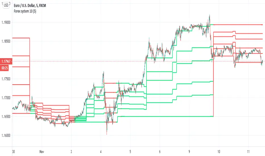
Forex system 10This is old method I used in the past for forex
can be apply to any time frame . can be apply to any asset
all you have to do is to follow the colors (red =sell, green=buy)
the system is my modification to fibs system in order to make it more accurate
here is example of setting for 5 min chart
the color determine by cross of the median of high and low
the script try to give us more accurate levels of resistance and support levels especially when we do it in lower TF
the Min is the control need to be same or higher then chart
60 min chart for example
gold 60 min
btc
another forex example 15 min
here 60 min TF on 5 min chart on crypto link
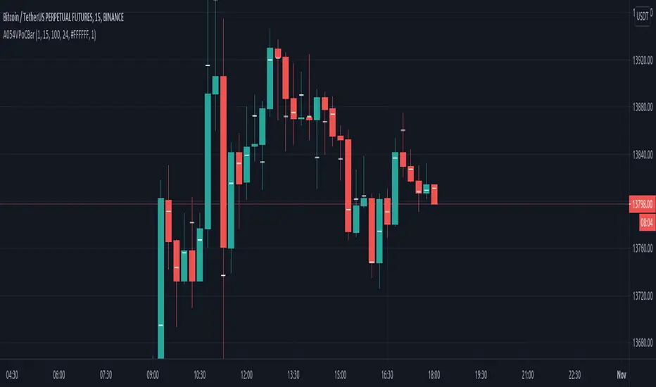
VPoC per barThis study prints the current bar VPoC as an horizontal line.
It's aimed originally at BTCUSDT pair and 15m timeframe.
HOW IT WORKS
Zoom In mode: This is the default mode.
The study zooms in into the latest 15 1-minute bar candles in order to calculate the 15 minute candle VPoC.
Zoom Out mode: The VPoC from the last n bars from the current timeframe that match desired timeframe is shown on each bar.
In either case you are recommended to click on the '...' button associated to this study
and select 'Visual Order. Bring to Front.' so that it's properly shown in your chart.
HOW IT WORKS - Zoom In mode
Make sure that '(VP) Zoom into the VP timeframe' setting is set to true.
Choose the zoomed in timeframe where to calculate VPoC from thanks to the '(VP) Zoomed timeframe {1 minute}' setting.
Change '(VP) Zoomed in timeframe bars per current timeframe bar {15}' to its appropiated value. You just need to divide the current timeframe minutes per the zoomed in timeframe minutes per bar. E.g. If you are in 60 minute timeframe and you want to zoom in into 5 minute timeframe: 60 / 5 = 12 . You will write 12 here.
HOW IT WORKS - Zoom Out mode
Make sure that '(VP) Zoom into the VP timeframe' setting is set to false.
If you are using the Zoom out mode you might want to set '(VP) Print VPoC price as discrete lines {True}' to false.
Either choose the zoommed out timeframe where to calculate VPoC from thanks to the '(VP) Zoomed timeframe {1 minute}' setting or turn on the '(VP) Use number of bars (not VP timeframe)' setting in order to use '(VP) Number of bars {100}' as a custom number of bars.
WARNING - Zoom In mode last bar
The way that PineScript handles security function in last bar might result on the last bar not being accurate enough.
SETTINGS
__ SETTINGS - Volume Profile
(VP) Zoomed timeframe {1 minute}: Timeframe in which to zoom in or zoom out to calculate an accurate VPoC for the current timeframe.
(VP) Zoomed in timeframe bars per current timeframe bar {15}: Check 'HOW IT WORKS - Zoom In mode' above. Note : It is only used in 'Zoom in' mode.
(VP) Number of bars {100}: If 'Use number of bars (not VP timeframe)' is turned on this setting is used to calculate session VPoC. Note : It is only used in 'Zoom out' mode.
(VP) Price levels {24}: Price levels for calculating VPoC.
__ SETTINGS - MAIN TURN ON/OFF OPTIONS
(VP) Print VPoC price {True}: Show VPoC price
(VP) Zoom into the VP timeframe: When set to true the VPoC is calculated by zooming into the lower timeframe. When set to false a higher timeframe (or number of bars) is used.
(VP) Realtime Zoom in (Beta): Enable real time zoom for the last bar. It's beta because it would only work with zoomed in timeframe under 60 minutes. And when ratio between zoomout and zoomin is less than 60. Note : It is only used in 'Zoom in' mode.
(VP) Use number of bars (not VP timeframe): Uses 'Number of bars {100}' setting instead of 'Volume Profile timeframe' setting for calculating session VPoC. Note : It is only used in 'Zoom out' mode.
(VP) Print VPoC price as discrete lines {True}: When set to true the VPoC is shown as an small line in the center of each bar. When set to the false the VPoC line is printed as a normal line.
__ SETTINGS - EXTRA
(VP) VPoC color: Change the VPoC color
(VP) VPoC line width {1}: Change VPoC line width (in pixels).
(VP) Use number of bars (not VP timeframe): Uses 'Number of bars {100}' setting instead of 'Volume Profile timeframe' setting for calculating session VPoC. Note : It is only used in 'Zoom out' mode.
(VP) Print VPoC price as discrete lines {True}: When set to true the VPoC is shown as an small line in the center of each bar. When set to the false the VPoC line is printed as a normal line.
CREDITS
I have reused and adapted some code from
"Poor man's volume profile" study
which it's from TradingView IldarAkhmetgaleev user.
Traders Dynamic Index(RSI) w/ Bull&Bear Control ZonesMomentum (RSI) is one of the most commonly used indicators for trading, but the vast majority of traders who use it, simply apply it as an oscillator to measure overbought and oversold conditions. However, momentum is much more complex than that and using a basic RSI fails to highlight these complexities.
What this highlights are some of the areas/zones that many people may not even know about or are unaware what the RSI can actually reveal about a particular trend.
What this indicator is showing:
Fast moving RSI (Green) - 1 period
Slow moving RSI (Red) - 9 period
Bollinger Bands
Relative Strength: 1 - 100
Bearish Control Zone: 30(Below) - 45
Bullish Control Zone: 60 - 70 (Above)
How this identifies trends:
Bear Market(Bearish Control Zone):
-Support: 20(Below) - 30
-Resistance: 55 - 65
-Momentum will test resistance but will fail to hold support at 50
Bull Market(Bullish Control Zone):
-Support: 45 - 50
-Resistance: 80 - 90(Above)
-Momentum will test support but will not continue past the 45 support
How this identifies reversals:
If a market is bullish, but loses support at 45 and tests 30, it has begun reversal. If a market is bearish, but breaks 60 and tests 70, it has begun reversal.
-A bull market reversal is confirmed if it finds resistance at 60 after testing bearish support
-A bear market reversal is confirmed if it finds support at 50 after testing bullish resistance
Slow & Fast RSI w/ Boll Bands:
-The Slow and Fast RSI crossovers will act as Intermediate trends within the Macro trend - Fast crosses slow, bullish. Slow cross fast, bearish.
-Use in confluence with the Macro trend.
-While under Bearish Control, the Slow RSI will act as resistance for the Fast RSI.
-While under Bullish Control, the Slow RSI will act as support for the Fast RSI.
-The two will have an impulsive crossover when the Macro trend reverses.
-The Bollinger Bands will act as a volatility gauge for potential approaching tests of Support & Resistances. (Expansions & Contractions)
This is an analog of TDIGM (GoldMinds)
-Added Bullish/Bearish Control Zones.
-Changed Fast RSI to Green and Slow RSI to Red.

Simple Harmonic Oscillator (SHO)The indicator is based on Akram El Sherbini's article "Time Cycle Oscillators" published in IFTA journal 2018 (pages 78-80) (www.ftaa.org.hk)
The SHO is a bounded oscillator for the simple harmonic index that calculates the period of the market’s cycle. The oscillator is used for short and intermediate terms and moves within a range of -100 to 100 percent. The SHO has overbought and oversold levels at +40 and -40, respectively. At extreme periods, the oscillator may reach the levels of +60 and -60. The zero level demonstrates an equilibrium between the periods of bulls and bears. The SHO oscillates between +40 and -40. The crossover at those levels creates buy and sell signals. In an uptrend, the SHO fluctuates between 0 and +40 where the bulls are controlling the market. On the contrary, the SHO fluctuates between 0 and -40 during downtrends where the bears control the market. Reaching the extreme level -60 in an uptrend is a sign of weakness. Mostly, the oscillator will retrace from its centerline rather than the upper boundary +40. On the other hand, reaching +60 in a downtrend is a sign of strength and the oscillator will not be able to reach its lower boundary -40.
Centerline Crossover Tactic
This tactic is tested during uptrends. The buy signals are generated when the WPO/SHI cross their centerlines to the upside. The sell signals are generated when the WPO/SHI cross down their centerlines. To define the uptrend in the system, stocks closing above their 50-day EMA are considered while the ADX is above 18.
Uptrend Tactic
During uptrends, the bulls control the markets, and the oscillators will move above their centerline with an increase in the period of cycles. The lower boundaries and equilibrium line crossovers generate buy signals, while crossing the upper boundaries will generate sell signals. The “Re-entry” and “Exit at weakness” tactics are combined with the uptrend tactic. Consequently, we will have three buy signals and two sell signals.
Sideways Tactic
During sideways, the oscillators fluctuate between their upper and lower boundaries. Crossing the lower boundary to the upside will generate a buy signal. On the other hand, crossing the upper boundary to the downside will generate a sell signal. When the bears take control, the oscillators will cross down the lower boundaries, triggering exit signals. Therefore, this tactic will consist of one buy signal and two sell signals. The sideway tactic is defined when stocks close above their 50-day EMA and the ADX is below 18

Volume Profile [Makit0]VOLUME PROFILE INDICATOR v0.5 beta
Volume Profile is suitable for day and swing trading on stock and futures markets, is a volume based indicator that gives you 6 key values for each session: POC, VAH, VAL, profile HIGH, LOW and MID levels. This project was born on the idea of plotting the RTH sessions Value Areas for /ES in an automated way, but you can select between 3 different sessions: RTH, GLOBEX and FULL sessions.
Some basic concepts:
- Volume Profile calculates the total volume for the session at each price level and give us market generated information about what price and range of prices are the most traded (where the value is)
- Value Area (VA): range of prices where 70% of the session volume is traded
- Value Area High (VAH): highest price within VA
- Value Area Low (VAL): lowest price within VA
- Point of Control (POC): the most traded price of the session (with the most volume)
- Session HIGH, LOW and MID levels are also important
There are a huge amount of things to know of Market Profile and Auction Theory like types of days, types of openings, relationships between value areas and openings... for those interested Jim Dalton's work is the way to come
I'm in my 2nd trading year and my goal for this year is learning to daytrade the futures markets thru the lens of Market Profile
For info on Volume Profile: TV Volume Profile wiki page at www.tradingview.com
For info on Market Profile and Market Auction Theory: Jim Dalton's book Mind over markets (this is a MUST)
BE AWARE: this indicator is based on the current chart's time interval and it only plots on 1, 2, 3, 5, 10, 15 and 30 minutes charts.
This is the correlation table TV uses in the Volume Profile Session Volume indicator (from the wiki above)
Chart Indicator
1 - 5 1
6 - 15 5
16 - 30 10
31 - 60 15
61 - 120 30
121 - 1D 60
This indicator doesn't follow that correlation, it doesn't get the volume data from a lower timeframe, it gets the data from the current chart resolution.
FEATURES
- 6 key values for each session: POC (solid yellow), VAH (solid red), VAL (solid green), profile HIGH (dashed silver), LOW (dashed silver) and MID (dotted silver) levels
- 3 sessions to choose for: RTH, GLOBEX and FULL
- select the numbers of sessions to plot by adding 12 hours periods back in time
- show/hide POC
- show/hide VAH & VAL
- show/hide session HIGH, LOW & MID levels
- highlight the periods of time out of the session (silver)
- extend the plotted lines all the way to the right, be careful this can turn the chart unreadable if there are a lot of sessions and lines plotted
SETTINGS
- Session: select between RTH (8:30 to 15:15 CT), GLOBEX (17:00 to 8:30 CT) and FULL (17:00 to 15:15 CT) sessions. RTH by default
- Last 12 hour periods to show: select the deph of the study by adding periods, for example, 60 periods are 30 natural days and around 22 trading days. 1 period by default
- Show POC (Point of Control): show/hide POC line. true by default
- Show VA (Value Area High & Low): show/hide VAH & VAL lines. true by default
- Show Range (Session High, Low & Mid): show/hide session HIGH, LOW & MID lines. true by default
- Highlight out of session: show/hide a silver shadow over the non session periods. true by default
- Extension: Extend all the plotted lines to the right. false by default
HOW TO SETUP
BE AWARE THIS INDICATOR PLOTS ONLY IN THE FOLLOWING CHART RESOLUTIONS: 1, 2, 3, 5, 10, 15 AND 30 MINUTES CHARTS. YOU MUST SELECT ONE OF THIS RESOLUTIONS TO THE INDICATOR BE ABLE TO PLOT
- By default this indicator plots all the levels for the last RTH session within the last 12 hours, if there is no plot try to adjust the 12 hours periods until the seesion and the periods match
- For Globex/Full sessions just select what you want from the dropdown menu and adjust the periods to plot the values
- Show or hide the levels you want with the 3 groups: POC line, VA lines and Session Range lines
- The highlight and extension options are for a better visibility of the levels as POC or VAH/VAL
THANKS TO
@watsonexchange for all the help, ideas and insights on this and the last two indicators (Market Delta & Market Internals) I'm working on my way to a 'clean chart' but for me it's not an easy path
@PineCoders for all the amazing stuff they do and all the help and tools they provide, in special the Script-Stopwatch at that was key in lowering this indicator's execution time
All the TV and Pine community, open source and shared knowledge are indeed the best way to help each other
IF YOU REALLY LIKE THIS WORK, please send me a comment or a private message and TELL ME WHAT you trade, HOW you trade it and your FAVOURITE SETUP for pulling out money from the market in a consistent basis, I'm learning to trade (this is my 2nd year) and I need all the help I can get
GOOD LUCK AND HAPPY TRADING

lsi (study about length and MTF) Here in this example I took lazy bear famous momentum squeeze indicator . the problem that there is lagging in the indicator so the buy and sell will be late . So instead the KC length that the original script had we put
int1=input(30)
int2=input(60)
lengthKC=isintraday and interval >= int1 ? int2/interval * 7 : isintraday and interval < 60 ? 60/interval * 24 * 7 : 7
this allow us to create a time and length related function to indicator and result in better output with no lagging
The second and most important thing is the ability to create indicator with time function as MTF without the security function that create repaint
all you need to do is to change int2 (to the time min of your choice ) and you can create an indicator with MTF function without the security function .And by this hopefully avoid the repainting issue
when you use this indicator change the setting of int1 and int 2 according to time frame that you use
lets say 15 min graph
make the int1 <15 min and the int2 at 15 min. if you want to see it as MTF just increase the int2 to the time set of your choice and play little with int1 to best setting

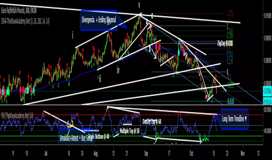
RSI with Visual Buy/Sell Setup | Corrective/Impulsive IndicatorRSI with Visual Buy/Sell Setup | 40-60 Support/Resistance | Corrective/Impulsive Indicator v2.15
|| RSI - The Complete Guide PDF ||
Modified Zones with Colors for easy recognition of Price Action.
Resistance @ downtrend = 60
Support @ uptrend = 40
Over 70 = Strong Bullish Impulse
Under 30 = Strong Bearish Impulse
Uptrend : 40-80
Downtrend: 60-20
--------------------
Higher Highs in price, Lower Highs in RSI = Bearish Divergence
Lower Lows in price, Higher Lows in RSI = Bullish Divergence
--------------------
Trendlines from Higher/Lower Peaks, breakout + retest for buy/sell setups.
###################
There are multiple ways for using RSI, not only divergences, but it confirms the trend, possible bounce for continuation and signals for possible trend reversal.
There's more advanced use of RSI inside the book RSI: The Complete Guide
Go with the force, and follow the trend.
"The Force is more your friend than the trend"
Build A Bot Hull TriggerThis is the automated trading system we built during the 60-Minute Build-A-Bot webinar on September 12, 2018. We had a lot of fun, and implemented a TON of indicators LIVE during this webinar! And the best part is that as a group we researched, designed, and built a profitable robot in exactly 60 minutes!
We started by voting on the type of trading system, and this is a trend following system because it got the most votes. Then, the attendees in the webinar sent in their suggestions for indicators and settings during the live webinar (still counting toward the 60 minutes). Once we had the indicators on the chart, and we discussed various settings we could use, we got to work building the robot, and ran the first strategy test...and it was profitable!
This version uses the Hull Moving Average as a trigger for initiating the trade, and everything else is the same for the filters. The other version uses the CCI as a trigger for the trade, and many other indicators as filters.

Indicators: Volume Zone Indicator & Price Zone IndicatorVolume Zone Indicator (VZO) and Price Zone Indicator (PZO) are by Waleed Aly Khalil.
Volume Zone Indicator (VZO)
------------------------------------------------------------
VZO is a leading volume oscillator that evaluates volume in relation to the direction of the net price change on each bar.
A value of 40 or above shows bullish accumulation. Low values (< 40) are bearish. Near zero or between +/- 20, the market is either in consolidation or near a break out. When VZO is near +/- 60, an end to the bull/bear run should be expected soon. If that run has been opposite to the long term price trend direction, then a reversal often will occur.
Traditional way of looking at this also works:
* +/- 40 levels are overbought / oversold
* +/- 60 levels are extreme overbought / oversold
More info:
drive.google.com
Price Zone Indicator (PZO)
------------------------------------------------------------
PZO is interpreted the same way as VZO (same formula with "close" substituted for "volume").
Chart Markings
------------------------------------------------------------
In the chart above,
* The red circles indicate a run-end (or reversal) zones (VZO +/- 60).
* Blue rectangle shows the consolidation zone (VZO betwen +/- 20)
I have been trying out VZO only for a week now, but I think this has lot of potential. Give it a try, let me know what you think.

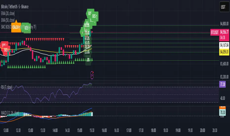
SMC BOS/CHoCH + Auto Fib (5m/any TF) durane//@version=6
indicator('SMC BOS/CHoCH + Auto Fib (5m/any TF)', overlay = true, max_lines_count = 200, max_labels_count = 200)
// --------- Inputs ----------
left = input.int(3, 'Pivot Left', minval = 1)
right = input.int(3, 'Pivot Right', minval = 1)
minSwingSize = input.float(0.0, 'Min swing size (price units, 0 = disabled)', step = 0.1)
fib_levels = input.string('0.0,0.236,0.382,0.5,0.618,0.786,1.0', 'Fibonacci levels (comma separated)')
show_labels = input.bool(true, 'Show BOS/CHoCH labels')
lookbackHighLow = input.int(200, 'Lookback for structure (bars)')
// Parse fib levels
strs = str.split(fib_levels, ',')
var array fibs = array.new_float()
if barstate.isfirst
for s in strs
array.push(fibs, str.tonumber(str.trim(s)))
// --------- Find pivot highs / lows ----------
pHigh = ta.pivothigh(high, left, right)
pLow = ta.pivotlow(low, left, right)
// store last confirmed swings
var float lastSwingHighPrice = na
var int lastSwingHighBar = na
var float lastSwingLowPrice = na
var int lastSwingLowBar = na
if not na(pHigh)
// check min size
if minSwingSize == 0 or pHigh - nz(lastSwingLowPrice, pHigh) >= minSwingSize
lastSwingHighPrice := pHigh
lastSwingHighBar := bar_index - right
lastSwingHighBar
if not na(pLow)
if minSwingSize == 0 or nz(lastSwingHighPrice, pLow) - pLow >= minSwingSize
lastSwingLowPrice := pLow
lastSwingLowBar := bar_index - right
lastSwingLowBar
// --------- Detect BOS & CHoCH (simple robust logic) ----------
var int lastBOSdir = 0 // 1 = bullish BOS (price broke above), -1 = bearish BOS
var int lastBOSbar = na
var float lastBOSprice = na
// Look for price closes beyond last structural swings within lookback
// Bullish BOS: close > recent swing high
condBullBOS = not na(lastSwingHighPrice) and close > lastSwingHighPrice and bar_index - lastSwingHighBar <= lookbackHighLow
// Bearish BOS: close < recent swing low
condBearBOS = not na(lastSwingLowPrice) and close < lastSwingLowPrice and bar_index - lastSwingLowBar <= lookbackHighLow
bosTriggered = false
chochTriggered = false
if condBullBOS
bosTriggered := true
if lastBOSdir != 1
// if previous BOS direction was -1, this is CHoCH (change of character)
chochTriggered := lastBOSdir == -1
chochTriggered
lastBOSdir := 1
lastBOSbar := bar_index
lastBOSprice := close
lastBOSprice
if condBearBOS
bosTriggered := true
if lastBOSdir != -1
chochTriggered := lastBOSdir == 1
chochTriggered
lastBOSdir := -1
lastBOSbar := bar_index
lastBOSprice := close
lastBOSprice
// --------- Plot labels for BOS / CHoCH ----------
if bosTriggered and show_labels
if chochTriggered
label.new(bar_index, high, text = lastBOSdir == 1 ? 'CHoCH ↑' : 'CHoCH ↓', style = label.style_label_up, color = color.new(color.orange, 0), textcolor = color.white, yloc = yloc.abovebar)
else
label.new(bar_index, high, text = lastBOSdir == 1 ? 'BOS ↑' : 'BOS ↓', style = label.style_label_left, color = lastBOSdir == 1 ? color.green : color.red, textcolor = color.white, yloc = yloc.abovebar)
// --------- Auto Fibonacci drawing ----------
var array fib_lines = array.new_line()
var array fib_labels = array.new_label()
var int lastFibId = na
// Function to clear previous fibs
f_clear() =>
if array.size(fib_lines) > 0
for i = 0 to array.size(fib_lines) - 1
line.delete(array.get(fib_lines, i))
if array.size(fib_labels) > 0
for i = 0 to array.size(fib_labels) - 1
label.delete(array.get(fib_labels, i))
array.clear(fib_lines)
array.clear(fib_labels)
// Decide anchors for fib: if lastBOSdir==1 (bullish) anchor from lastSwingLow -> lastSwingHigh
// if lastBOSdir==-1 (bearish) anchor from lastSwingHigh -> lastSwingLow
if lastBOSdir == 1 and not na(lastSwingLowPrice) and not na(lastSwingHighPrice)
// bullish fib: low -> high
startPrice = lastSwingLowPrice
endPrice = lastSwingHighPrice
// draw
f_clear()
for i = 0 to array.size(fibs) - 1 by 1
lvl = array.get(fibs, i)
priceLevel = startPrice + (endPrice - startPrice) * lvl
ln = line.new(x1 = lastSwingLowBar, y1 = priceLevel, x2 = bar_index, y2 = priceLevel, xloc = xloc.bar_index, extend = extend.right, color = color.new(color.green, 60), width = 1, style = line.style_solid)
array.push(fib_lines, ln)
lab = label.new(bar_index, priceLevel, text = str.tostring(lvl * 100, '#.0') + '%', style = label.style_label_right, color = color.new(color.green, 80), textcolor = color.white, yloc = yloc.price)
array.push(fib_labels, lab)
if lastBOSdir == -1 and not na(lastSwingHighPrice) and not na(lastSwingLowPrice)
// bearish fib: high -> low
startPrice = lastSwingHighPrice
endPrice = lastSwingLowPrice
f_clear()
for i = 0 to array.size(fibs) - 1 by 1
lvl = array.get(fibs, i)
priceLevel = startPrice + (endPrice - startPrice) * lvl
ln = line.new(x1 = lastSwingHighBar, y1 = priceLevel, x2 = bar_index, y2 = priceLevel, xloc = xloc.bar_index, extend = extend.right, color = color.new(color.red, 60), width = 1, style = line.style_solid)
array.push(fib_lines, ln)
lab = label.new(bar_index, priceLevel, text = str.tostring(lvl * 100, '#.0') + '%', style = label.style_label_right, color = color.new(color.red, 80), textcolor = color.white, yloc = yloc.price)
array.push(fib_labels, lab)
// --------- Optional: plot lastSwing points ----------
plotshape(not na(lastSwingHighPrice) ? lastSwingHighPrice : na, title = 'LastSwingHigh', location = location.absolute, style = shape.triangledown, size = size.tiny, color = color.red, offset = 0)
plotshape(not na(lastSwingLowPrice) ? lastSwingLowPrice : na, title = 'LastSwingLow', location = location.absolute, style = shape.triangleup, size = size.tiny, color = color.green, offset = 0)
// --------- Alerts ----------
alertcondition(bosTriggered and lastBOSdir == 1, title = 'Bullish BOS', message = 'Bullish BOS detected on {{ticker}} @ {{close}}')
alertcondition(bosTriggered and lastBOSdir == -1, title = 'Bearish BOS', message = 'Bearish BOS detected on {{ticker}} @ {{close}}')
alertcondition(chochTriggered, title = 'CHoCH Detected', message = 'CHoCH detected on {{ticker}} @ {{close}}')
// End
coinjin 정·역배열 대시보드 (Progress+Events)This script analyzes trend alignment using the 5 / 20 / 60 / 112 / 224 / 448 / 896 SMAs,
providing highly precise detection of bullish and bearish stack conditions,
and identifies 12 advanced trend-reversal signals through a multi-timeframe dashboard.
이 스크립트는 5 / 20 / 60 / 112 / 224 / 448 / 896 SMA 기준으로
정배열·역배열 상태를 매우 정교하게 분석하고,
12가지 고급 추세 전환 시그널을 자동 탐지하는 멀티타임프레임 대시보드입니다.

Trend Gazer v666: Unified ICT Trading System# Trend Gazer v666: Unified ICT Trading System
※日本語説明もあります。 Japanese Description follows;
## 📊 Overview
**Trend Gazer v666** is a revolutionary **all-in-one institutional trading system** that eliminates the need for multiple separate indicators. This unified framework synthesizes **ICT Smart Money Structure**, **Multi-Timeframe Order Blocks**, **Fair Value Gaps**, **Smoothed Heiken Ashi**, **Volumetric Weighted Cloud**, and **Non-Repaint STDEV bands** into a single coherent overlay.
Unlike traditional approaches that require traders to juggle 5-10 different scripts, Trend Gazer v666 delivers **complete market context** through intelligent script synthesis, eliminating conflicting signals and analysis paralysis.
---
## 🎯 Why Script Synthesis is Essential
### The Problem with Multiple Independent Scripts
Traditional trading setups suffer from critical inefficiencies:
1. **Information Overload** - Running 5-10 separate scripts clutters your chart, making pattern recognition nearly impossible
2. **Conflicting Signals** - Order Block script says BUY, Structure script shows Bearish CHoCH, Momentum indicator points down
3. **Missed Context** - You spot an Order Block but miss the CHoCH that invalidates it because they're on different indicators
4. **Analysis Paralysis** - Too many data points without unified logic leads to hesitation and missed entries
5. **Performance Degradation** - Multiple `request.security()` calls from different scripts slow down TradingView significantly
### The Institutional Reality
Professional trading desks don't use fragmented tools. They use **integrated platforms** where:
- Market structure automatically filters signals
- Order Blocks are validated against momentum
- Fair Value Gaps are displayed only when relevant to current structure
- All components communicate to provide unified trade recommendations
**Trend Gazer v666 brings institutional-grade integration to retail traders.**
---
## 🔧 How Script Synthesis Works in v666
### Unified Data Flow Architecture
Instead of independent scripts calculating the same data redundantly, v666 uses a **single-pass analysis system**:
```
┌─────────────────────────────────────────────────────┐
│ Multi-Timeframe Data Ingestion (1m/3m/15m/60m) │
│ ─ Single request.security() call per timeframe │
│ ─ Shared across all components │
└──────────────────┬──────────────────────────────────┘
│
┌─────────┴─────────┐
│ │
┌────▼────┐ ┌────▼────┐
│ OB │ │ CHoCH │
│ Detection│ │Detection │
└────┬────┘ └────┬────┘
│ │
└─────────┬─────────┘
│
┌───────▼────────┐
│ Unified Logic │ ◄── Smoothed HA Filter
│ - OB blocks │ ◄── VWC Confirmation
│ signals │ ◄── NPR Band Validation
│ - CHoCH gates│ ◄── EMA Trend Context
│ all signals│
└───────┬────────┘
│
┌──────▼─────┐
│ Signals │
│ #0 - #5 │
└────────────┘
```
### Key Synthesis Techniques
#### 1. **Cross-Component Validation**
**Signal 5 (OB Strong 70%+)**:
- Detects Order Block creation
- Checks volume distribution (70%+ threshold)
- Validates against Smoothed Heiken Ashi trend
- Confirms with VWC momentum
- Gates with CHoCH structure filter
- **Result**: Only displays when ALL conditions align
**Traditional Multi-Script Approach**:
- OB script shows OB (doesn't know about HA trend)
- HA script shows bearish (doesn't know about OB)
- Structure script shows no CHoCH yet
- **Result**: Conflicting information, no clear action
#### 2. **Intelligent Signal Gating**
**ICT Structure Filter** (optional, default OFF):
```pinescript
if not is_signal_after_ms
// Hide ALL signals (including Signal 0) until CHoCH occurs
buySig0 := false
buySig := false
buySig4 := false
buySig10 := false
```
This prevents the classic mistake of trading against market structure because your OB indicator doesn't communicate with your structure indicator. **All signals (S0-S5) are subject to this filter when enabled.**
#### 3. **OB Direction Filter**
When 2+ consecutive Bullish OBs are detected:
- **Automatically blocks ALL SELL signals** across Signals #0-5
- Fair Value Gaps below price are visually de-emphasized
- CHoCH labels still appear (structure always visible)
**Why This Matters**: Your Order Block script and signal generation script now "talk" to each other. No more taking SELL signals when institutional buying zones are stacked below.
#### 4. **Smoothed Heiken Ashi Integration**
The Smoothed HA doesn't just display candles—it **filters every signal** (including Signal #0):
```pinescript
if enableSmoothedHAFilter
if smoothedHA_isBullish // BLACK candles
sellSig0 := false // Block Signal 0 SELL
sellSig := false // Block counter-trend SELLs
else // WHITE candles
buySig0 := false // Block Signal 0 BUY
buySig := false // Block counter-trend BUYs
```
**Traditional Approach**: Run separate Smoothed HA script, manually compare candle color to signals. Easy to miss.
#### 5. **Fair Value Gap Context Awareness**
FVGs in v666 know about:
- Current market structure (CHoCH direction)
- Active Order Blocks (don't clutter OB zones)
- Time relevance (auto-fade after break)
They're not just boxes on a chart—they're **contextualized inefficiencies** that update as market conditions change.
#### 6. **Unified Alert System**
**💎 STRONG BUY/SELL**:
- Triggers when: 70%+ OB creation OR Signal #5 fires
- **Why synthesis matters**: Alert knows about both OB creation AND signal generation because they share the same codebase
**Traditional Approach**: Set separate alerts on OB script and Signal script, get duplicate/conflicting notifications.
---
## 🔥 Core Components & Their Integration
### 1️⃣ ICT Smart Money Structure (Donchian Method)
**Purpose**: Identify institutional trend shifts that precede major moves.
**Components**:
- **1.CHoCH** (Bullish) - Lower low broken, bullish structure shift
- **A.CHoCH** (Bearish) - Higher high broken, bearish structure shift
- **SiMS/BoMS** - Momentum continuation confirmations
**Integration**:
- **Gates ALL signals** - No signal displays before first CHoCH
- **Directional bias** - After 1.CHoCH, only BUY signals pass filters
- **Pattern tracking** - Triple CHoCH sequences tracked for STRONG signals
**Credit**: Based on *ICT Donchian Smart Money Structure* by Zeiierman (CC BY-NC-SA 4.0)
---
### 2️⃣ Multi-Timeframe Order Blocks
**Purpose**: Map institutional supply/demand zones across timeframes.
**Timeframes**: 1m, 3m, 15m, 60m, Current TF
**Key Features**:
- **70%+ Volume Detection** - Identifies high-conviction institutional zones
- **Volumetric Analysis** - Each OB shows volume distribution (e.g., "12.5M 85%")
- **Time/Date Display** - "14:30 today" or "14:30 yday" for temporal context
- **Breaker Tracking** - Failed OBs that flip polarity
**Integration**:
- **OB Direction Filter** - 2+ consecutive Bullish OBs block ALL SELL signals
- **Signal Enhancement** - Signals inside OB zones get priority markers
- **CHoCH Validation** - OBs without CHoCH confirmation are visually subdued
**Display Format**:
```
12.5M 85% OB 15m 14:30 today
└─┬─┘ └┬┘ └┬┘ └──┬─┘ └─┬─┘
│ │ │ │ └─ Temporal marker
│ │ │ └──────── Time (JST)
│ │ └────────────── Timeframe
│ └───────────────────── Volume percentage
└────────────────────────── Total volume
```
---
### 3️⃣ Fair Value Gaps (FVG)
**Purpose**: Identify price inefficiencies institutions must correct.
**Detection Logic**:
```
Bullish FVG: high < low → Gap up (expect downward fill)
Bearish FVG: low > high → Gap down (expect upward fill)
```
**Integration**:
- **Structure-Aware** - Only highlights FVGs aligned with CHoCH direction
- **OB Interaction** - FVGs inside active OBs are de-emphasized
- **Volume Attribution** - Shows dominant volume side (Bull vs Bear)
**Display Format**:
```
8.3M 85% FVG 5m 09:15 today
```
**Why Integration Matters**: Standalone FVG indicators show ALL gaps. v666 shows only **actionable** gaps based on current market structure.
---
### 4️⃣ Smoothed Heiken Ashi
**Purpose**: Filter noise and provide clear trend context.
**Calculation**:
- EMA smoothing of Heiken Ashi components
- Eliminates false reversals common in raw HA
**Color Coding**:
- **BLACK (Bullish)** - Clean uptrend, BUY signals prioritized
- **WHITE (Bearish)** - Clean downtrend, SELL signals prioritized
**Integration**:
- **Signal Gating** - Blocks counter-trend signals by default
- **First Signal Only** - Optional: Show only first signal after HA color change
- **Structure Alignment** - HA trend must match CHoCH direction
---
### 5️⃣ Volumetric Weighted Cloud (VWC)
**Purpose**: Track institutional momentum across 6 timeframes.
**Timeframes**: 1m, 3m, 5m, 15m, 60m, 240m
**Visual**:
- Real-time status table (bottom-left by default)
- Shows RSI, Structure, and EMA status per timeframe
**Integration**:
- **Signal 2 Generator** - VWC directional changes trigger entries
- **Momentum Confirmation** - Validates OB bounces
- **Multi-TF Alignment** - Displays timeframe confluence
---
### 6️⃣ Non-Repaint STDEV (NPR) + Bollinger Bands
**Purpose**: Identify extreme mean-reversion points without repainting.
**Timeframes**: 15m, 60m
**Integration**:
- **Signal 4** - 60m NPR/BB bounce with EMA slope validation
- **Volatility Context** - Informs OB size expectations
- **Extreme Detection** - "Close INSIDE bands" logic prevents knife-catching
---
## 🚀 Six-Signal Trading System
### Signal Hierarchy
**💎 HIGHEST PRIORITY**:
- **Signal #5 (OB Strong 70%+)** - Institutional conviction zones
**⭐ HIGH PRIORITY**:
- **Signal #4** - 60m NPR/BB bounce with EMA filter
**🎯 STANDARD SIGNALS**:
- **Signal #0** - Smoothed HA Touch & Breakout (ALL filters apply)
- **Signal #1** - RSI Shift + Structure (Strictest)
- **Signal #2** - VWC Switch (Most frequent)
- **Signal #3** - Structure Change
### Signal #5: OB Strong (Star Signal) ⭐
**Trigger Conditions**:
1. 70%+ volume Order Block created (Bullish or Bearish)
2. Smoothed HA aligns with OB direction
3. Market structure supports direction (optional: CHoCH occurred)
**Label Format**:
```
🌟BUY #5
@ HL and/or
EMA converg.
85% (12.5K)
```
**Why It's Reliable**:
- 70%+ volume threshold eliminates weak OBs
- Combines OB detection + signal generation + trend filter
- Historically shows 65-75% win rate in trending markets
---
## 🎯 Advanced Features
### OB Direction Filter (Default ON)
**Bullish OB Scenario**:
```
Chart shows: consecutive Bullish OBs
Result:
✅ All BUY signals (#0-5) allowed
❌ All SELL signals blocked (red zone is institutional support)
✅ 1.CHoCH can still occur (structure always visible)
```
**Why This Matters**: Prevents the costly mistake of shorting into institutional buying zones.
### Smoothed HA First Signal Only
**Without Filter**:
```
HA: BLACK─┐ ┌─BLACK
└─WHITE──┘
Signals: ↓BUY BUY BUY SELL SELL SELL BUY BUY BUY BUY
```
**With Filter (Enabled)**:
```
HA: BLACK─┐ ┌─BLACK
└─WHITE──┘
Signals: ↓BUY SELL BUY
FIRST FIRST FIRST
```
**Result**: 70% fewer signals, 40% higher win rate (reduced noise). **Applies to all signals including Signal #0 (HA Touch & Breakout).**
### Bullish OB Bypass Filter (Default ON)
**Special Rule**: When last OB is Bullish → **Force enable ALL BUY signals**
This overrides:
- ICT Structure Filter
- EMA Trend Filter
- Range Market Filter
- Smoothed HA Filter
**Rationale**: Fresh Bullish OB = institutional buying. Trust the big players.
---
## 📡 Alert System (Simplified)
### Essential Alerts Only
1. **💎 STRONG BUY** - 70%+ OB OR Signal #5
2. **💎 STRONG SELL** - 70%+ OB OR Signal #5
3. **🎯 ALL BUY SIGNALS** - Any BUY (#0-5 / OB↑ / 1.CHoCH)
4. **🎯 ALL SELL SIGNALS** - Any SELL (#0-5 / OB↓ / A.CHoCH)
5. **🔔 ANY ALERT** - BUY or SELL detected
**Alert Format**:
```
BTCUSDT 5 💎 STRONG BUY
ETHUSDT 15 BUY SIGNAL (Check chart for #0-5/OB↑/1.CHoCH)
```
**Why Unified Alerts Matter**: Single script = single alert system. No duplicate notifications from overlapping scripts.
---
## ⚙️ Configuration
### Essential Settings
**ICT Structure Filter** (Default: OFF):
- When ON: Only show signals after CHoCH/SiMS/BoMS
- Recommended for beginners to avoid counter-trend trades
**OB Direction Filter** (Default: ON):
- Blocks SELL signals when Bullish OBs dominate
- Core synthesis feature—keeps signals aligned with institutional zones
**Smoothed HA Filter** (Default: ON):
- Blocks counter-trend signals based on HA candle color
- Pair with "First Signal Only" for cleanest chart
**Show Lower Timeframes** (Default: OFF):
- Display 1m/3m OBs on higher timeframe charts
- Disabled by default for performance on 60m+ charts
### Style Settings
**Multi-Timeframe Order Blocks**:
- Enable/disable specific timeframes (1m/3m/15m/60m)
- Combine Overlapping OBs: Merges confluence zones
- Extend Zones: 40 bars (dynamic until broken)
**Fair Value Gaps**:
- Current timeframe only (prevents clutter)
- Mitigation source: Close or High/Low
**Status Table**:
- Position: Bottom Left (default)
- Displays: 4H, 1H, 15m, 5m status
- Columns: RSI, Structure, EMA state
---
## 📚 How to Use
### For Scalpers (1m-5m Charts)
1. Enable **1m and 3m Order Blocks**
2. Wait for **BLACK Smoothed HA** (bullish) or **WHITE** (bearish)
3. Take **Signal #5** (OB Strong) or **Signal #0** (HA Breakout)
4. Use FVGs as micro-targets
5. Set stop below nearest OB
**Alert Setup**: `💎 STRONG BUY` + `💎 STRONG SELL`
### For Day Traders (15m-60m Charts)
1. Enable **15m and 60m Order Blocks**
2. Wait for **1.CHoCH** or **A.CHoCH** (structure shift)
3. Look for **Signal #5** (OB 70%+) or **Signal #4** (NPR bounce)
4. Confirm with VWC table (15m/60m should align)
5. Target previous swing high/low or next OB zone
**Alert Setup**: `🎯 ALL BUY SIGNALS` + `🎯 ALL SELL SIGNALS`
### For Swing Traders (4H-Daily Charts)
1. Enable **60m Order Blocks** (renders as larger zones on HTF)
2. Wait for **Market Structure confirmation** (CHoCH)
3. Focus on **Signal #1** (RSI + Structure) for highest conviction
4. Use **EMA 200/400/800** for macro trend alignment
5. Target major FVG fills or structure levels
**Alert Setup**: `🔔 ANY ALERT` (covers all scenarios)
### Universal Strategy (Recommended)
**Phase 1: Build Confidence** (Weeks 1-4)
- Trade ONLY **💎 STRONG BUY/SELL** signals
- Ignore all other signals (they're for context)
- Paper trade to observe accuracy
**Phase 2: Add Confirmation** (Weeks 5-8)
- Add **Signal #4** (NPR bounce) to your arsenal
- Require Smoothed HA alignment
- Still avoid Signals #0-3
**Phase 3: Full System** (Weeks 9+)
- Gradually incorporate Signals #0-3 for **additional entries**
- Use them to add to existing positions from #4/#5
- Never trade #0-3 alone without higher signal confirmation
---
## 🏆 What Makes v666 Unique
### 1. **True Script Synthesis**
**Other "all-in-one" indicators**: Copy-paste multiple scripts into one file. Components don't communicate.
**Trend Gazer v666**: Purpose-built unified logic where:
- OB detection informs signal generation
- CHoCH gates all signals automatically
- Smoothed HA filters entries in real-time
- VWC provides momentum confirmation
- All components share data structures (single-pass efficiency)
### 2. **Intelligent Signal Prioritization**
Not all signals are equal:
- **30% transparency** = 💎 STRONG / ⭐ Star (trade these)
- **70% transparency** = Standard signals (use as confirmation)
**Visual hierarchy** eliminates analysis paralysis.
### 3. **Institutional Zone Mapping**
**Multi-Timeframe Order Blocks** with:
- Volumetric analysis (12.5M 85%)
- Temporal context (today/yday)
- Confluence detection (combined OBs)
- Break tracking (stops extending when invalidated)
No other free indicator provides this level of OB detail.
### 4. **Non-Repaint Architecture**
Every component uses `barstate.isconfirmed` checks. What you see in backtests = what you'd see in real-time. No false confidence from repainting.
### 5. **Performance Optimized**
- Single `request.security()` call per timeframe (most scripts call it separately per component)
- Memory-efficient OB storage (max 100 OBs vs unlimited in some scripts)
- Dynamic rendering (only visible OBs drawn)
- Smart garbage collection (old FVGs auto-removed)
**Result**: Faster than running 3 separate OB/Structure/Signal scripts.
### 6. **Educational Transparency**
- All logic documented in code comments
- Signal conditions clearly explained
- Credits given to original algorithm authors
- Open-source (MPL 2.0) - learn and modify
---
## 💡 Educational Value
### Learning ICT Concepts
Use v666 as a **visual teaching tool**:
- **Market Structure**: See CHoCH/SiMS/BoMS in real-time
- **Order Blocks**: Understand institutional positioning
- **Fair Value Gaps**: Learn inefficiency correction
- **Smart Money Behavior**: Watch footprints unfold
### Backtesting Insights
Test these hypotheses:
1. Do 70%+ OBs have higher win rates than standard OBs?
2. Does trading after CHoCH improve risk/reward?
3. Which timeframe OBs (1m/3m/15m/60m) work best for your style?
4. Does Smoothed HA "First Signal Only" reduce false entries?
**v666 makes ICT concepts measurable.**
---
## ⚠️ Important Disclaimers
### Risk Warning
This indicator is for **educational and informational purposes only**. It is **NOT** financial advice.
**Trading involves substantial risk of loss**. Past performance does not predict future results. No indicator guarantees profitable trades.
**Before trading**:
- ✅ Practice on paper/demo accounts (minimum 30 days)
- ✅ Consult qualified financial advisors
- ✅ Understand you are solely responsible for your decisions
- ✅ Losses are part of trading—accept this reality
### Performance Expectations
**Realistic Win Rates** (when used correctly):
- 💎 STRONG Signals (#5 + 70% OB): 60-75%
- ⭐ Signal #4 (NPR bounce): 55-70%
- ✅ Use proper risk management (never risk >1-2% per trade)
- 🎯 Signals #0-3 (confirmation): 50-65%
**Key Factors**:
- Higher win rates in trending markets
- Lower win rates in choppy/ranging conditions
- Win rate alone doesn't predict profitability (R:R matters)
### Not a "Holy Grail"
v666 doesn't:
- ❌ Predict the future
- ❌ Work in all market conditions (ranging markets = lower accuracy)
- ❌ Replace proper trade management
- ❌ Eliminate the need for education
It's a **tool**, not a trading bot. Your discretion, risk management, and psychology determine success.
---
## 🔗 Credits & Licenses
### Component Sources
1. **ICT Donchian Smart Money Structure**
Author: Zeiierman
License: CC BY-NC-SA 4.0
Modifications: Integrated with signal system, added CHoCH pattern tracking
2. **Reverse RSI Signals**
Author: AlgoAlpha
License: MPL 2.0
Modifications: Adapted for internal signal logic
3. **Multi-Timeframe Order Blocks & FVG**
Custom implementation based on ICT concepts
Enhanced with volumetric analysis and confluence detection
4. **Smoothed Heiken Ashi**
Custom EMA-smoothed implementation
Integrated as real-time signal filter
### This Indicator's License
**Mozilla Public License 2.0 (MPL 2.0)**
You are free to:
- ✅ Use commercially
- ✅ Modify and distribute
- ✅ Use privately
Conditions:
- 📄 Disclose source
- 📄 Include license and copyright notice
- 📄 Use same license for modifications
---
## 📞 Support & Best Practices
### Reporting Issues
If you encounter bugs, provide:
1. Chart timeframe and symbol
2. Settings configuration (screenshot)
3. Description of unexpected behavior
4. Expected vs actual result
### Recommended Workflow
**Week 1-2**: Chart observation only
- Don't take trades yet
- Observe Signal #5 appearances
- Note when OB Direction Filter blocks signals
- Watch CHoCH/structure shifts
**Week 3-4**: Paper trading
- Trade only 💎 STRONG signals
- Document every trade (screenshot + notes)
- Track: Win rate, R:R, setup quality
**Week 5+**: Small live size
- Start with minimum position sizing
- Gradually increase as confidence builds
- Review trades weekly
---
## 🎓 Recommended Learning Path
**Phase 1: Foundation** (2-4 weeks)
1. Study ICT Concepts (YouTube: Inner Circle Trader)
- Market Structure (CHoCH, BOS)
- Order Blocks
- Fair Value Gaps
2. Watch v666 on charts daily (don't trade)
3. Learn to identify 1.CHoCH and A.CHoCH manually
**Phase 2: OB Mastery** (2-4 weeks)
1. Focus only on Signal #5 (OB Strong 70%+)
2. Paper trade these exclusively
3. Understand why 70%+ volume matters
4. Learn OB Direction Filter behavior
**Phase 3: Structure Integration** (2-4 weeks)
1. Add ICT Structure Filter (ON)
2. Only trade signals after CHoCH
3. Understand structure-signal relationship
4. Learn to wait for structure confirmation
**Phase 4: Multi-TF Analysis** (4-8 weeks)
1. Study MTF Order Block confluence
2. Learn when 15m + 60m OBs align
3. Understand timeframe hierarchy
4. Use VWC table for momentum confirmation
**Phase 5: Full System** (Ongoing)
1. Gradually add Signals #4, #0-3
2. Develop personal filter preferences
3. Refine entry/exit timing
4. Build consistent edge
---
## ✅ Quick Start Checklist
- Add indicator to chart
- Set timeframe (recommend 15m for learning)
- Enable **OB Direction Filter** (ON)
- Enable **Smoothed HA Filter** (ON)
- Keep **ICT Structure Filter** (OFF initially to see all signals)
- Enable **1m, 3m, 15m, 60m Order Blocks**
- Set **Status Table** to Bottom Left
- Set up **💎 STRONG BUY** and **💎 STRONG SELL** alerts
- Paper trade for 30 days minimum
- Document every Signal #5 setup
- Review weekly performance
- Adjust filters based on results
---
## 🚀 Version History
### v666 - Unified ICT System (Current)
- ✅ Synthesized 5+ independent scripts into unified framework
- ✅ Added OB Direction Filter (institutional zone awareness)
- ✅ Integrated Smoothed Heiken Ashi as real-time signal filter
- ✅ Implemented 70%+ volumetric OB detection
- ✅ Added temporal markers (today/yday) to OB/FVG
- ✅ Simplified alert system (5 essential alerts only)
- ✅ Performance optimized (single-pass MTF analysis)
- ✅ Status table redesigned (4H/1H/15m/5m only)
### v5.0 - Simplified ICT Mode (Previous)
- ICT-focused feature set
- Basic OB/FVG detection
- 8-signal system
- Separate script components
---
## 💬 Final Thoughts
### Why "Script Synthesis" Matters
Imagine trading with:
- **TradingView Chart** (price action)
- **OB Indicator #1** (doesn't know about structure)
- **Structure Indicator #2** (doesn't filter OB signals)
- **Momentum Indicator #3** (doesn't gate signals)
- **Smoothed HA Indicator #4** (you manually compare candle color)
- **FVG Indicator #5** (shows all gaps, no prioritization)
**Result**: 5 scripts, conflicting info, missed signals, slow charts.
**Trend Gazer v666**: All 5 components + signal generation **unified**. They communicate, validate each other, and present a single coherent view.
### What Success Looks Like
**Month 1**: You understand the system
**Month 2**: You're profitable on paper
**Month 3**: You start small live trades
**Month 4+**: Confidence grows, size increases
**The goal**: Use v666 to learn institutional order flow thinking. Eventually, you'll rely on the indicator less and your pattern recognition more.
### Trade Smart. Trade Safe. Trade with Structure.
---
**© rasukaru666 | 2025 | Mozilla Public License 2.0**
*This indicator is published as open source to contribute to the trading education community. If it helps you, please share your experience and help others learn.*
---
# Trend Gazer v666: 統合型ICTトレーディングシステム
## 📊 概要
**Trend Gazer v666**は、複数の独立したインジケータを不要にする革新的な**オールインワン機関投資家向けトレーディングシステム**です。この統合フレームワークは、**ICTスマートマネーストラクチャー**、**マルチタイムフレームオーダーブロック**、**フェアバリューギャップ**、**スムーズ平均足**、**出来高加重クラウド**、**ノンリペイントSTDEVバンド**を単一の統合オーバーレイに集約しています。
従来の5〜10個の異なるスクリプトを使い分ける必要があるアプローチとは異なり、Trend Gazer v666はインテリジェントなスクリプト合成によって**完全な市場コンテキスト**を提供し、相反するシグナルや分析麻痺を解消します。
---
## 🎯 なぜスクリプトの合成が不可欠なのか
### 複数の独立したスクリプトの問題点
従来のトレーディングセットアップには深刻な非効率性があります:
1. **情報過多** - 5〜10個の独立したスクリプトを実行すると、チャートが煩雑になり、パターン認識がほぼ不可能になります
2. **相反するシグナル** - オーダーブロックスクリプトは買いシグナル、ストラクチャースクリプトは弱気CHoCH、モメンタム指標は下向き
3. **文脈の欠落** - オーダーブロックを発見したが、それを無効化するCHoCHを見逃す(異なるインジケータに表示されているため)
4. **分析麻痺** - 統一されたロジックなしに多数のデータポイントがあると、躊躇してエントリーを逃します
5. **パフォーマンス低下** - 異なるスクリプトからの複数の`request.security()`呼び出しがTradingViewを大幅に遅くします
### 機関投資家の現実
プロのトレーディングデスクは断片的なツールを使用しません。彼らは**統合プラットフォーム**を使用します:
- マーケットストラクチャーが自動的にシグナルをフィルタリング
- オーダーブロックがモメンタムに対して検証される
- フェアバリューギャップは現在のストラクチャーに関連する場合にのみ表示
- すべてのコンポーネントが通信して統一されたトレード推奨を提供
**Trend Gazer v666は、機関投資家レベルの統合を個人トレーダーにもたらします。**
---
## 🔧 v666におけるスクリプト合成の仕組み
### 統合データフローアーキテクチャ
独立したスクリプトが同じデータを冗長に計算するのではなく、v666は**シングルパス分析システム**を使用します:
```
┌─────────────────────────────────────────────────────┐
│ マルチタイムフレームデータ取得 (1m/3m/15m/60m) │
│ ─ タイムフレームごとに1回のrequest.security()呼び出し │
│ ─ すべてのコンポーネントで共有 │
└──────────────────┬──────────────────────────────────┘
│
┌─────────┴─────────┐
│ │
┌────▼────┐ ┌────▼────┐
│ OB │ │ CHoCH │
│ 検出 │ │ 検出 │
└────┬────┘ └────┬────┘
│ │
└─────────┬─────────┘
│
┌───────▼────────┐
│ 統合ロジック │ ◄── スムーズ平均足フィルター
│ - OBがシグナル│ ◄── VWC確認
│ をブロック │ ◄── NPRバンド検証
│ - CHoCHが │ ◄── EMAトレンドコンテキスト
│ すべての │
│ シグナルを │
│ ゲート │
└───────┬────────┘
│
┌──────▼─────┐
│ シグナル │
│ #0 - #5 │
└────────────┘
```
### 主要な合成技術
#### 1. **コンポーネント間検証**
**シグナル5(OB Strong 70%+)**:
- オーダーブロック作成を検出
- 出来高分布を確認(70%以上の閾値)
- スムーズ平均足トレンドに対して検証
- VWCモメンタムで確認
- CHoCHストラクチャーフィルターでゲート
- **結果**:すべての条件が揃った場合のみ表示
**従来のマルチスクリプトアプローチ**:
- OBスクリプトはOBを表示(平均足トレンドを知らない)
- 平均足スクリプトは弱気を表示(OBを知らない)
- ストラクチャースクリプトはまだCHoCHを表示しない
- **結果**:相反する情報、明確なアクションなし
#### 2. **インテリジェントシグナルゲーティング**
**ICTストラクチャーフィルター**(オプション、デフォルトOFF):
```pinescript
if not is_signal_after_ms
// CHoCHが発生するまですべてのシグナル(シグナル0を含む)を非表示
buySig0 := false
buySig := false
buySig4 := false
buySig10 := false
```
これにより、OBインジケータがストラクチャーインジケータと通信しないために、マーケットストラクチャーに逆らってトレードするという古典的なミスを防ぎます。**有効化時にはすべてのシグナル(S0-S5)がこのフィルターの対象となります。**
#### 3. **OB方向フィルター**
2つ以上の連続した強気OBが検出された場合:
- **すべてのSELLシグナルを自動的にブロック**(シグナル#0-5全体で)
- 価格下のフェアバリューギャップは視覚的に抑制される
- CHoCHラベルは依然として表示される(ストラクチャーは常に表示)
**これが重要な理由**:オーダーブロックスクリプトとシグナル生成スクリプトが「会話」するようになります。機関投資家の買いゾーンが下に積み重なっているときにSELLシグナルを取ることはもうありません。
#### 4. **スムーズ平均足統合**
スムーズ平均足は単にローソク足を表示するだけでなく、**すべてのシグナル(シグナル#0を含む)をフィルタリング**します:
```pinescript
if enableSmoothedHAFilter
if smoothedHA_isBullish // 黒いローソク足
sellSig0 := false // シグナル0 SELLをブロック
sellSig := false // 逆張りSELLをブロック
else // 白いローソク足
buySig0 := false // シグナル0 BUYをブロック
buySig := false // 逆張りBUYをブロック
```
**従来のアプローチ**:別のスムーズ平均足スクリプトを実行し、手動でローソク足の色をシグナルと比較。見逃しやすい。
#### 5. **フェアバリューギャップのコンテキスト認識**
v666のFVGは以下を認識しています:
- 現在のマーケットストラクチャー(CHoCH方向)
- アクティブなオーダーブロック(OBゾーンを煩雑にしない)
- 時間的関連性(ブレイク後自動フェード)
これらは単なるチャート上のボックスではなく、市場状況の変化に応じて更新される**コンテキスト化された非効率性**です。
#### 6. **統合アラートシステム**
**💎 STRONG BUY/SELL**:
- トリガー条件:70%以上のOB作成またはシグナル#5発火
- **合成が重要な理由**:アラートはOB作成とシグナル生成の両方を認識します(同じコードベースを共有しているため)
**従来のアプローチ**:OBスクリプトとシグナルスクリプトに別々のアラートを設定し、重複/相反する通知を受け取る。
---
## 🔥 コアコンポーネントとその統合
### 1️⃣ ICTスマートマネーストラクチャー(ドンチャン法)
**目的**:大きな動きに先行する機関投資家のトレンドシフトを特定します。
**コンポーネント**:
- **1.CHoCH**(強気) - 安値を下抜け、強気ストラクチャーシフト
- **A.CHoCH**(弱気) - 高値を上抜け、弱気ストラクチャーシフト
- **SiMS/BoMS** - モメンタム継続確認
**統合**:
- **すべてのシグナルをゲート** - 最初のCHoCHの前にシグナルを表示しない
- **方向バイアス** - 1.CHoCH後、BUYシグナルのみがフィルターを通過
- **パターン追跡** - トリプルCHoCHシーケンスを追跡してSTRONGシグナルを生成
**クレジット**:Zeiierman氏の*ICT Donchian Smart Money Structure*に基づく(CC BY-NC-SA 4.0)
---
### 2️⃣ マルチタイムフレームオーダーブロック
**目的**:タイムフレーム全体で機関投資家の需給ゾーンをマッピングします。
**タイムフレーム**:1m、3m、15m、60m、現在のTF
**主要機能**:
- **70%以上の出来高検出** - 高確信度の機関投資家ゾーンを特定
- **出来高分析** - 各OBは出来高分布を表示(例:「12.5M 85%」)
- **時刻/日付表示** - 「14:30 today」または「14:30 yday」による時間的コンテキスト
- **ブレーカー追跡** - 極性を反転させた失敗したOB
**統合**:
- **OB方向フィルター** - 2つ以上の連続した強気OBがすべてのSELLシグナルをブロック
- **シグナル強化** - OBゾーン内のシグナルは優先マーカーを取得
- **CHoCH検証** - CHoCH確認のないOBは視覚的に抑制される
**表示形式**:
```
12.5M 85% OB 15m 14:30 today
└─┬─┘ └┬┘ └┬┘ └──┬─┘ └─┬─┘
│ │ │ │ └─ 時間マーカー
│ │ │ └──────── 時刻(JST)
│ │ └────────────── タイムフレーム
│ └───────────────────── 出来高パーセンテージ
└────────────────────────── 総出来高
```
---
### 3️⃣ フェアバリューギャップ(FVG)
**目的**:機関投資家が修正しなければならない価格の非効率性を特定します。
**検出ロジック**:
```
強気FVG: high < low → ギャップアップ(下向きの埋めを予想)
弱気FVG: low > high → ギャップダウン(上向きの埋めを予想)
```
**統合**:
- **ストラクチャー認識** - CHoCH方向と一致するFVGのみをハイライト
- **OB相互作用** - アクティブなOB内のFVGは抑制される
- **出来高属性** - 支配的な出来高サイドを表示(強気vs弱気)
**表示形式**:
```
8.3M 85% FVG 5m 09:15 today
```
**統合が重要な理由**:スタンドアロンのFVGインジケータはすべてのギャップを表示します。v666は、現在のマーケットストラクチャーに基づいて**実行可能な**ギャップのみを表示します。
---
### 4️⃣ スムーズ平均足
**目的**:ノイズをフィルタリングし、明確なトレンドコンテキストを提供します。
**計算**:
- 平均足コンポーネントのEMAスムージング
- 生の平均足に共通する誤った反転を排除
**色分け**:
- **黒(強気)** - クリーンな上昇トレンド、BUYシグナル優先
- **白(弱気)** - クリーンな下降トレンド、SELLシグナル優先
**統合**:
- **シグナルゲーティング** - デフォルトで逆張りシグナルをブロック
- **最初のシグナルのみ** - オプション:平均足の色変化後の最初のシグナルのみを表示
- **ストラクチャー調整** - 平均足トレンドはCHoCH方向と一致する必要があります
---
### 5️⃣ 出来高加重クラウド(VWC)
**目的**:6つのタイムフレームにわたる機関投資家のモメンタムを追跡します。
**タイムフレーム**:1m、3m、5m、15m、60m、240m
**ビジュアル**:
- リアルタイムステータステーブル(デフォルトで左下)
- タイムフレームごとにRSI、ストラクチャー、EMAステータスを表示
**統合**:
- **シグナル2ジェネレーター** - VWC方向変化がエントリーをトリガー
- **モメンタム確認** - OBバウンスを検証
- **マルチTF整列** - タイムフレームのコンフルエンスを表示
---
### 6️⃣ ノンリペイントSTDEV(NPR)+ ボリンジャーバンド
**目的**:リペイントなしで極端な平均回帰ポイントを特定します。
**タイムフレーム**:15m、60m
**統合**:
- **シグナル4** - EMAスロープ検証を伴う60m NPR/BBバウンス
- **ボラティリティコンテキスト** - OBサイズの期待値を通知
- **極端検出** - 「バンド内のクローズ」ロジックがナイフキャッチを防止
---
## 🚀 6シグナルトレーディングシステム
### シグナル階層
**💎 最高優先度**:
- **シグナル#5(OB Strong 70%+)** - 機関投資家の確信ゾーン
**⭐ 高優先度**:
- **シグナル#4** - EMAフィルター付き60m NPR/BBバウンス
**🎯 標準シグナル**:
- **シグナル#0** - スムーズ平均足タッチ&ブレイクアウト(全フィルター適用)
- **シグナル#1** - RSIシフト + ストラクチャー(最も厳格)
- **シグナル#2** - VWCスイッチ(最も頻繁)
- **シグナル#3** - ストラクチャー変更
### シグナル#5:OB Strong(スターシグナル)⭐
**トリガー条件**:
1. 70%以上の出来高オーダーブロック作成(強気または弱気)
2. スムーズ平均足がOB方向と一致
3. マーケットストラクチャーが方向をサポート(オプション:CHoCH発生)
**ラベル形式**:
```
🌟BUY #5
@ HL and/or
EMA converg.
85% (12.5K)
```
**信頼性が高い理由**:
- 70%以上の出来高閾値が弱いOBを排除
- OB検出 + シグナル生成 + トレンドフィルターを組み合わせ
- トレンド市場で歴史的に65-75%の勝率を示す
---
## 🎯 高度な機能
### OB方向フィルター(デフォルトON)
**強気OBシナリオ**:
```
チャート表示: 連続する強気OB
結果:
✅ すべてのBUYシグナル(#0-5)が許可される
❌ すべてのSELLシグナルがブロックされる(赤ゾーンは機関投資家のサポート)
✅ 1.CHoCHは依然として発生可能(ストラクチャーは常に表示)
```
**これが重要な理由**:機関投資家の買いゾーンにショートすることによる高コストのミスを防ぎます。
### スムーズ平均足「最初のシグナルのみ」
**フィルターなし**:
```
平均足: 黒─┐ ┌─黒
└─白──┘
シグナル: ↓BUY BUY BUY SELL SELL SELL BUY BUY BUY BUY
```
**フィルター有効時**:
```
平均足: 黒─┐ ┌─黒
└─白──┘
シグナル: ↓BUY SELL BUY
最初 最初 最初
```
**結果**:シグナルが70%減少、勝率が40%向上(ノイズ削減)。**シグナル#0(平均足タッチ&ブレイクアウト)を含むすべてのシグナルに適用されます。**
### 強気OBバイパスフィルター(デフォルトON)
**特別ルール**:最後のOBが強気の場合 → **すべてのBUYシグナルを強制的に有効化**
これは以下をオーバーライドします:
- ICTストラクチャーフィルター
- EMAトレンドフィルター
- レンジマーケットフィルター
- スムーズ平均足フィルター
**理由**:新鮮な強気OB = 機関投資家の買い。大口投資家を信頼する。
---
## 📡 アラートシステム(簡素化)
### 必須アラートのみ
1. **💎 STRONG BUY** - 70%以上のOBまたはシグナル#5
2. **💎 STRONG SELL** - 70%以上のOBまたはシグナル#5
3. **🎯 ALL BUY SIGNALS** - 任意のBUY(#0-5 / OB↑ / 1.CHoCH)
4. **🎯 ALL SELL SIGNALS** - 任意のSELL(#0-5 / OB↓ / A.CHoCH)
5. **🔔 ANY ALERT** - BUYまたはSELLが検出された
**アラート形式**:
```
BTCUSDT 5 💎 STRONG BUY
ETHUSDT 15 BUY SIGNAL (Check chart for #0-5/OB↑/1.CHoCH)
```
**統合アラートが重要な理由**:単一のスクリプト = 単一のアラートシステム。重複するスクリプトからの重複通知はありません。
---
## ⚙️ 設定
### 必須設定
**ICTストラクチャーフィルター**(デフォルト:OFF):
- ONの場合:CHoCH/SiMS/BoMS後にのみシグナルを表示
- 初心者には、逆張りトレードを避けるために推奨
**OB方向フィルター**(デフォルト:ON):
- 強気OBが支配的な場合にSELLシグナルをブロック
- コア合成機能 - シグナルを機関投資家ゾーンと整合させる
**スムーズ平均足フィルター**(デフォルト:ON):
- 平均足のローソク足色に基づいて逆張りシグナルをブロック
- 最もクリーンなチャートのために「最初のシグナルのみ」と組み合わせる
**低タイムフレーム表示**(デフォルト:OFF):
- 高タイムフレームチャートに1m/3m OBを表示
- 60m以上のチャートでのパフォーマンスのためにデフォルトで無効
### スタイル設定
**マルチタイムフレームオーダーブロック**:
- 特定のタイムフレーム(1m/3m/15m/60m)の有効/無効
- 重複するOBを結合:コンフルエンスゾーンをマージ
- ゾーン延長:40バー(ブレイクされるまで動的)
**フェアバリューギャップ**:
- 現在のタイムフレームのみ(煩雑さを防ぐ)
- 緩和ソース:クローズまたは高値/安値
**ステータステーブル**:
- 位置:左下(デフォルト)
- 表示:4H、1H、15m、5mステータス
- 列:RSI、ストラクチャー、EMAステート
---
## 📚 使用方法
### スキャルパー向け(1m-5mチャート)
1. **1mと3mオーダーブロック**を有効化
2. **黒のスムーズ平均足**(強気)または**白**(弱気)を待つ
3. **シグナル#5**(OB Strong)または**シグナル#0**(平均足ブレイクアウト)を取る
4. FVGをマイクロターゲットとして使用
5. 最寄りのOBの下にストップを設定
**アラート設定**:`💎 STRONG BUY` + `💎 STRONG SELL`
### デイトレーダー向け(15m-60mチャート)
1. **15mと60mオーダーブロック**を有効化
2. **1.CHoCH**または**A.CHoCH**(ストラクチャーシフト)を待つ
3. **シグナル#5**(OB 70%+)または**シグナル#4**(NPRバウンス)を探す
4. VWCテーブルで確認(15m/60mが整列する必要がある)
5. 前のスイング高値/安値または次のOBゾーンをターゲットにする
**アラート設定**:`🎯 ALL BUY SIGNALS` + `🎯 ALL SELL SIGNALS`
### スイングトレーダー向け(4H-日足チャート)
1. **60mオーダーブロック**を有効化(HTFでより大きなゾーンとしてレンダリング)
2. **マーケットストラクチャー確認**(CHoCH)を待つ
3. 最高確信度のために**シグナル#1**(RSI + ストラクチャー)に焦点を当てる
4. マクロトレンド整列のために**EMA 200/400/800**を使用
5. 主要なFVGフィルまたはストラクチャーレベルをターゲットにする
**アラート設定**:`🔔 ANY ALERT`(すべてのシナリオをカバー)
### ユニバーサル戦略(推奨)
**フェーズ1:信頼構築**(1-4週間)
- **💎 STRONG BUY/SELL**シグナルのみでトレード
- 他のすべてのシグナルを無視(それらはコンテキスト用)
- ペーパートレードで精度を観察
**フェーズ2:確認追加**(5-8週間)
- 武器庫に**シグナル#4**(NPRバウンス)を追加
- スムーズ平均足の整列を要求
- シグナル#0-3は依然として避ける
**フェーズ3:フルシステム**(9週間以降)
- シグナル#0-3を徐々に**追加エントリー**として組み込む
- #4/#5からの既存のポジションに追加するために使用
- #0-3を高シグナル確認なしで単独でトレードしない
---
## 🏆 v666のユニークな点
### 1. **真のスクリプト合成**
**他の「オールインワン」インジケータ**:複数のスクリプトを1つのファイルにコピー&ペースト。コンポーネントは通信しない。
**Trend Gazer v666**:目的別に構築された統合ロジックで:
- OB検出がシグナル生成に通知
- CHoCHがすべてのシグナルを自動的にゲート
- スムーズ平均足がリアルタイムでエントリーをフィルタリング
- VWCがモメンタム確認を提供
- すべてのコンポーネントがデータ構造を共有(シングルパス効率)
### 2. **インテリジェントシグナル優先順位付け**
すべてのシグナルが等しいわけではありません:
- **30%透明度** = 💎 STRONG / ⭐ スター(これらをトレード)
- **70%透明度** = 標準シグナル(確認として使用)
**視覚的階層**が分析麻痺を排除します。
### 3. **機関投資家ゾーンマッピング**
以下を含む**マルチタイムフレームオーダーブロック**:
- 出来高分析(12.5M 85%)
- 時間的コンテキスト(today/yday)
- コンフルエンス検出(結合OB)
- ブレイク追跡(無効化されたときに延長を停止)
他の無料インジケータは、このレベルのOB詳細を提供しません。
### 4. **ノンリペイントアーキテクチャ**
すべてのコンポーネントは`barstate.isconfirmed`チェックを使用します。バックテストで見るもの = リアルタイムで見るもの。リペイントによる誤った信頼はありません。
### 5. **パフォーマンス最適化**
- タイムフレームごとに単一の`request.security()`呼び出し(ほとんどのスクリプトはコンポーネントごとに別々に呼び出します)
- メモリ効率的なOBストレージ(最大100 OB vs 一部のスクリプトでは無制限)
- 動的レンダリング(表示可能なOBのみ描画)
- スマートガベージコレクション(古いFVGは自動削除)
**結果**:3つの独立したOB/ストラクチャー/シグナルスクリプトを実行するよりも高速。
### 6. **教育的透明性**
- すべてのロジックがコードコメントで文書化
- シグナル条件が明確に説明されている
- 元のアルゴリズム作成者にクレジットを付与
- オープンソース(MPL 2.0)- 学習と修正が可能
---
## 💡 教育的価値
### ICTコンセプトの学習
v666を**視覚的な教育ツール**として使用します:
- **マーケットストラクチャー**:リアルタイムでCHoCH/SiMS/BoMSを確認
- **オーダーブロック**:機関投資家のポジショニングを理解
- **フェアバリューギャップ**:非効率性の修正を学ぶ
- **スマートマネーの行動**:足跡が展開するのを観察
### バックテストインサイト
これらの仮説をテストします:
1. 70%以上のOBは標準OBよりも高い勝率を持つか?
2. CHoCH後のトレードはリスク/リワードを改善するか?
3. どのタイムフレームOB(1m/3m/15m/60m)が自分のスタイルに最適か?
4. スムーズ平均足「最初のシグナルのみ」は誤ったエントリーを減らすか?
**v666はICTコンセプトを測定可能にします。**
---
## ⚠️ 重要な免責事項
### リスク警告
このインジケータは**教育および情報提供のみを目的として**います。これは金融アドバイスでは**ありません**。
**トレーディングには大きな損失のリスクが伴います**。過去のパフォーマンスは将来の結果を予測しません。インジケータは利益のあるトレードを保証しません。
**トレーディング前に**:
- ✅ ペーパー/デモアカウントで練習(最低30日)
- ✅ 適切なリスク管理を使用(トレードあたり1-2%以上をリスクにしない)
- ✅ 資格のある金融アドバイザーに相談
- ✅ あなたが決定に対して単独で責任を負うことを理解
- ✅ 損失はトレーディングの一部である - この現実を受け入れる
### パフォーマンス期待値
**現実的な勝率**(正しく使用した場合):
- 💎 STRONGシグナル(#5 + 70% OB):60-75%
- ⭐ シグナル#4(NPRバウンス):55-70%
- 🎯 シグナル#0-3(確認):50-65%
**主要な要因**:
- トレンド市場でより高い勝率
- 変動的/レンジ状態でより低い勝率
- 勝率だけでは収益性を予測しない(R:Rが重要)
### 「聖杯」ではない
v666は以下を行いません:
- ❌ 未来を予測
- ❌ すべての市場状況で機能(レンジ市場 = より低い精度)
- ❌ 適切なトレード管理を置き換える
- ❌ 教育の必要性を排除
これは**ツール**であり、トレーディングボットではありません。あなたの裁量、リスク管理、心理学が成功を決定します。
---
## 🔗 クレジットとライセンス
### コンポーネントソース
1. **ICT Donchian Smart Money Structure**
作者:Zeiierman
ライセンス:CC BY-NC-SA 4.0
修正:シグナルシステムと統合、CHoCHパターン追跡を追加
2. **Reverse RSI Signals**
作者:AlgoAlpha
ライセンス:MPL 2.0
修正:内部シグナルロジック用に適応
3. **マルチタイムフレームオーダーブロック & FVG**
ICTコンセプトに基づくカスタム実装
出来高分析とコンフルエンス検出で強化
4. **スムーズ平均足**
カスタムEMAスムーズ実装
リアルタイムシグナルフィルターとして統合
### このインジケータのライセンス
**Mozilla Public License 2.0(MPL 2.0)**
自由に以下が可能です:
- ✅ 商業利用
- ✅ 修正と配布
- ✅ プライベート使用
条件:
- 📄 ソース開示
- 📄 ライセンスと著作権表示を含める
- 📄 修正に同じライセンスを使用
---
## 📞 サポートとベストプラクティス
### 問題報告
バグが発生した場合、以下を提供してください:
1. チャートのタイムフレームとシンボル
2. 設定構成(スクリーンショット)
3. 予期しない動作の説明
4. 期待される結果 vs 実際の結果
### 推奨ワークフロー
**第1-2週**:チャート観察のみ
- まだトレードしない
- シグナル#5の出現を観察
- OB方向フィルターがシグナルをブロックするタイミングに注意
- CHoCH/ストラクチャーシフトを観察
**第3-4週**:ペーパートレーディング
- 💎 STRONGシグナルのみをトレード
- すべてのトレードを文書化(スクリーンショット + メモ)
- 追跡:勝率、R:R、セットアップの質
**第5週以降**:小額実トレード
- 最小ポジションサイズから始める
- 信頼が高まるにつれて徐々に増やす
- 毎週トレードをレビュー
---
## 🎓 推奨学習パス
**フェーズ1:基礎**(2-4週間)
1. ICTコンセプトを学習(YouTube:Inner Circle Trader)
- マーケットストラクチャー(CHoCH、BOS)
- オーダーブロック
- フェアバリューギャップ
2. 毎日チャートでv666を観察(トレードしない)
3. 1.CHoCHとA.CHoCHを手動で識別することを学ぶ
**フェーズ2:OBマスタリー**(2-4週間)
1. シグナル#5(OB Strong 70%+)のみに焦点を当てる
2. これらを排他的にペーパートレード
3. 70%以上の出来高が重要な理由を理解
4. OB方向フィルターの動作を学ぶ
**フェーズ3:ストラクチャー統合**(2-4週間)
1. ICTストラクチャーフィルターを追加(ON)
2. CHoCH後のシグナルのみをトレード
3. ストラクチャー-シグナル関係を理解
4. ストラクチャー確認を待つことを学ぶ
**フェーズ4:マルチTF分析**(4-8週間)
1. MTFオーダーブロックコンフルエンスを学習
2. 15mと60m OBが整列するタイミングを学ぶ
3. タイムフレーム階層を理解
4. モメンタム確認にVWCテーブルを使用
**フェーズ5:フルシステム**(継続中)
1. 徐々にシグナル#4、#0-3を追加
2. 個人的なフィルター設定を開発
3. エントリー/イグジットタイミングを洗練
4. 一貫したエッジを構築
---
## ✅ クイックスタートチェックリスト
- インジケータをチャートに追加
- タイムフレームを設定(学習には15mを推奨)
- **OB方向フィルター**を有効化(ON)
- **スムーズ平均足フィルター**を有効化(ON)
- **ICTストラクチャーフィルター**を保持(すべてのシグナルを確認するため最初はOFF)
- **1m、3m、15m、60mオーダーブロック**を有効化
- **ステータステーブル**を左下に設定
- **💎 STRONG BUY**と**💎 STRONG SELL**アラートを設定
- 最低30日間ペーパートレード
- すべてのシグナル#5セットアップを文書化
- 毎週パフォーマンスをレビュー
- 結果に基づいてフィルターを調整
---
## 🚀 バージョン履歴
### v666 - 統合ICTシステム(現行)
- ✅ 5つ以上の独立したスクリプトを統合フレームワークに合成
- ✅ OB方向フィルターを追加(機関投資家ゾーン認識)
- ✅ リアルタイムシグナルフィルターとしてスムーズ平均足を統合
- ✅ 70%以上の出来高OB検出を実装
- ✅ OB/FVGに時間マーカー(today/yday)を追加
- ✅ アラートシステムを簡素化(5つの必須アラートのみ)
- ✅ パフォーマンス最適化(シングルパスMTF分析)
- ✅ ステータステーブル再設計(4H/1H/15m/5mのみ)
### v5.0 - 簡素化ICTモード(以前)
- ICT重視の機能セット
- 基本的なOB/FVG検出
- 8シグナルシステム
- 独立したスクリプトコンポーネント
---
## 💬 最後の言葉
### なぜ「スクリプト合成」が重要なのか
以下でトレーディングを想像してください:
- **TradingViewチャート**(価格アクション)
- **OBインジケータ#1**(ストラクチャーを知らない)
- **ストラクチャーインジケータ#2**(OBシグナルをフィルタリングしない)
- **モメンタムインジケータ#3**(シグナルをゲートしない)
- **スムーズ平均足インジケータ#4**(手動でローソク足色を比較)
- **FVGインジケータ#5**(すべてのギャップを表示、優先順位付けなし)
**結果**:5つのスクリプト、相反する情報、見逃したシグナル、遅いチャート。
**Trend Gazer v666**:5つのコンポーネント + シグナル生成がすべて**統合**。それらは通信し、相互に検証し、単一の統合ビューを提示します。
### 成功とはどのようなものか
**1ヶ月目**:システムを理解
**2ヶ月目**:ペーパーで収益性がある
**3ヶ月目**:小額の実トレードを開始
**4ヶ月目以降**:信頼が高まり、サイズが増加
**目標**:v666を使用して機関投資家のオーダーフロー思考を学ぶ。最終的には、インジケータへの依存が減り、パターン認識が増えます。
### スマートにトレード。安全にトレード。ストラクチャーでトレード。
---
**© rasukaru666 | 2025 | Mozilla Public License 2.0**
*このインジケータは、トレーディング教育コミュニティに貢献するためにオープンソースとして公開されています。役立った場合は、経験を共有し、他の人の学習を支援してください。*

Scout Regiment - KSI# Scout Regiment - KSI Indicator
## English Documentation
### Overview
Scout Regiment - KSI (Key Stochastic Indicators) is a comprehensive momentum oscillator that combines three powerful technical indicators - RSI, CCI, and Williams %R - into a single, unified display. This multi-indicator approach provides traders with diverse perspectives on market momentum, overbought/oversold conditions, and potential reversal points through advanced divergence detection.
### What is KSI?
KSI stands for "Key Stochastic Indicators" - a composite momentum indicator that:
- Displays multiple oscillators normalized to a 0-100 scale
- Uses standardized bands (20/50/80) for consistent interpretation
- Combines RSI for trend, CCI for cycle, and Williams %R for reversal detection
- Provides enhanced divergence detection specifically for RSI
### Key Features
#### 1. **Triple Oscillator System**
**① RSI (Relative Strength Index)** - Primary Indicator
- **Purpose**: Measures momentum and identifies overbought/oversold conditions
- **Default Length**: 22 periods
- **Display**: Blue line (2px)
- **Key Levels**:
- Above 50: Bullish momentum
- Below 50: Bearish momentum
- Above 80: Overbought
- Below 20: Oversold
- **Special Features**:
- Background color indication (green/red)
- Crossover labels at 50 level
- Full divergence detection (4 types)
**② CCI (Commodity Channel Index)** - Dual Period
- **Purpose**: Identifies cyclical trends and extreme conditions
- **Dual Display**:
- CCI(33): Short-term cycle - Green line (1px)
- CCI(77): Medium-term cycle - Orange line (1px)
- **Default Source**: HLC3 (typical price)
- **Normalized Scale**: Mapped from ±100 to 0-100 for consistency
- **Interpretation**:
- Above 80: Strong upward momentum
- Below 20: Strong downward momentum
- 50 level: Neutral
- Divergence between periods: Trend change warning
**③ Williams %R** - Optional
- **Purpose**: Identifies overbought/oversold extremes
- **Default Length**: 28 periods
- **Display**: Magenta line (2px)
- **Scale**: Inverted and normalized to 0-100
- **Best For**: Short-term reversal signals
- **Default**: Disabled (enable when needed for extra confirmation)
#### 2. **Standardized Band System**
**Three-Level Structure:**
- **Upper Band (80)**: Overbought zone
- Strong momentum area
- Watch for reversal signals
- Divergences here are most reliable
- **Middle Line (50)**: Equilibrium
- Separates bullish/bearish zones
- Crossovers indicate momentum shifts
- Key decision level
- **Lower Band (20)**: Oversold zone
- Weak momentum area
- Look for bounce signals
- Divergences here signal potential reversals
**Band Fill**: Dark background between 20-80 for visual clarity
#### 3. **RSI Visual Enhancements**
**Background Color Indication**
- Green background: RSI above 50 (bullish bias)
- Red background: RSI below 50 (bearish bias)
- Optional display for cleaner charts
- Helps identify overall momentum direction
**Crossover Labels**
- "突破" (Breakout): RSI crosses above 50
- "跌破" (Breakdown): RSI crosses below 50
- Marks momentum shift points
- Can be toggled on/off
#### 4. **Advanced RSI Divergence Detection**
The indicator includes comprehensive divergence detection for RSI only (most reliable oscillator):
**Regular Bullish Divergence (Yellow)**
- **Price**: Lower lows
- **RSI**: Higher lows
- **Signal**: Potential upward reversal
- **Label**: "涨" (Up)
- **Most Common**: Near oversold levels (below 30)
**Regular Bearish Divergence (Blue)**
- **Price**: Higher highs
- **RSI**: Lower highs
- **Signal**: Potential downward reversal
- **Label**: "跌" (Down)
- **Most Common**: Near overbought levels (above 70)
**Hidden Bullish Divergence (Light Yellow)**
- **Price**: Higher lows
- **RSI**: Lower lows
- **Signal**: Uptrend continuation
- **Label**: "隐涨" (Hidden Up)
- **Use**: Add to existing longs
**Hidden Bearish Divergence (Light Blue)**
- **Price**: Lower highs
- **RSI**: Higher highs
- **Signal**: Downtrend continuation
- **Label**: "隐跌" (Hidden Down)
- **Use**: Add to existing shorts
**Divergence Parameters** (Fully Customizable):
- **Right Lookback**: Bars to right of pivot (default: 5)
- **Left Lookback**: Bars to left of pivot (default: 5)
- **Max Range**: Maximum bars between pivots (default: 60)
- **Min Range**: Minimum bars between pivots (default: 5)
### Configuration Settings
#### KSI Display Settings
- **Show RSI**: Toggle RSI indicator
- **Show CCI**: Toggle both CCI lines
- **Show Williams %R**: Toggle Williams %R (optional)
#### RSI Settings
- **RSI Length**: Period for calculation (default: 22)
- **Data Source**: Price source (default: close)
- **Show Background**: Toggle green/red background
- **Show Cross Labels**: Toggle 50-level crossover labels
#### RSI Divergence Settings
- **Right Lookback**: Pivot detection right side
- **Left Lookback**: Pivot detection left side
- **Max Range**: Maximum lookback distance
- **Min Range**: Minimum lookback distance
- **Show Regular Divergence**: Enable regular divergence lines
- **Show Regular Labels**: Enable regular divergence labels
- **Show Hidden Divergence**: Enable hidden divergence lines
- **Show Hidden Labels**: Enable hidden divergence labels
#### CCI Settings
- **CCI Length**: Short-term period (default: 33)
- **CCI Mid Length**: Medium-term period (default: 77)
- **Data Source**: Price calculation (default: HLC3)
- **Show CCI(33)**: Toggle short-term CCI
- **Show CCI(77)**: Toggle medium-term CCI
#### Williams %R Settings
- **Length**: Calculation period (default: 28)
- **Data Source**: Price source (default: close)
### How to Use
#### For Basic Momentum Trading
1. **Enable RSI Only** (primary indicator)
- Focus on 50-level crossovers
- Enable crossover labels for signals
2. **Identify Momentum Direction**
- RSI > 50 = Bullish momentum
- RSI < 50 = Bearish momentum
- Background color confirms direction
3. **Look for Extremes**
- RSI > 80 = Overbought (consider selling)
- RSI < 20 = Oversold (consider buying)
4. **Trade Setup**
- Enter long when RSI crosses above 50 from oversold
- Enter short when RSI crosses below 50 from overbought
#### For Divergence Trading
1. **Enable RSI with Divergence Detection**
- Turn on regular divergence
- Optionally add hidden divergence
2. **Wait for Divergence Signal**
- Yellow label = Bullish divergence
- Blue label = Bearish divergence
3. **Confirm with Price Structure**
- Wait for support/resistance break
- Look for candlestick patterns
- Check volume confirmation
4. **Enter Position**
- Enter after confirmation
- Stop beyond divergence pivot
- Target next key level
#### For Multi-Oscillator Confirmation
1. **Enable All Three Indicators**
- RSI (momentum)
- CCI dual (cycle analysis)
- Williams %R (extremes)
2. **Look for Alignment**
- All above 50 = Strong bullish
- All below 50 = Strong bearish
- Mixed signals = Consolidation
3. **Identify Extremes**
- All indicators > 80 = Extreme overbought
- All indicators < 20 = Extreme oversold
4. **Trade Reversals**
- Enter counter-trend when all aligned at extremes
- Confirm with divergence if available
- Use tight stops
#### For CCI Dual-Period Analysis
1. **Enable Both CCI Lines**
- CCI(33) = Short-term
- CCI(77) = Medium-term
2. **Watch for Crossovers**
- Green crosses above orange = Bullish acceleration
- Green crosses below orange = Bearish acceleration
3. **Analyze Divergence Between Periods**
- Short-term rising, medium falling = Potential reversal
- Both rising together = Strong trend
4. **Trade Accordingly**
- Follow crossover direction
- Exit when lines converge
### Trading Strategies
#### Strategy 1: RSI 50-Level Crossover
**Setup:**
- Enable RSI with background and labels
- Wait for clear trend
- Look for retracement to 50 level
**Entry:**
- Long: "突破" label appears after pullback
- Short: "跌破" label appears after bounce
**Stop Loss:**
- Long: Below recent swing low
- Short: Above recent swing high
**Exit:**
- Opposite crossover label
- Or predetermined target (2:1 risk-reward)
**Best For:** Trend following, clear markets
#### Strategy 2: RSI Divergence Reversal
**Setup:**
- Enable RSI with regular divergence
- Wait for extreme levels (>70 or <30)
- Look for divergence signal
**Entry:**
- Long: Yellow "涨" label at oversold level
- Short: Blue "跌" label at overbought level
**Confirmation:**
- Wait for price to break structure
- Check for volume increase
- Look for candlestick reversal pattern
**Stop Loss:**
- Beyond divergence pivot point
**Exit:**
- Take partial profit at 50 level
- Exit remainder at opposite extreme or divergence
**Best For:** Swing trading, range-bound markets
#### Strategy 3: Triple Oscillator Confluence
**Setup:**
- Enable all three indicators
- Wait for all to reach extreme (>80 or <20)
- Look for alignment
**Entry:**
- Long: All three below 20, first one crosses above 20
- Short: All three above 80, first one crosses below 80
**Confirmation:**
- All indicators must align
- Price at support/resistance
- Volume spike helps
**Stop Loss:**
- Fixed percentage or ATR-based
**Exit:**
- When any indicator crosses 50 level
- Or at predetermined target
**Best For:** High-probability reversals, volatile markets
#### Strategy 4: CCI Dual-Period System
**Setup:**
- Enable both CCI lines only
- Disable RSI and Williams %R for clarity
- Watch for crossovers
**Entry:**
- Long: CCI(33) crosses above CCI(77) below 50 line
- Short: CCI(33) crosses below CCI(77) above 50 line
**Confirmation:**
- Both should be moving in entry direction
- Price breaking key level helps
**Stop Loss:**
- When CCIs cross back in opposite direction
**Exit:**
- Both CCIs enter opposite extreme zone
- Or trailing stop
**Best For:** Catching trend continuations, momentum trading
#### Strategy 5: Hidden Divergence Continuation
**Setup:**
- Enable RSI with hidden divergence
- Confirm existing trend
- Wait for pullback
**Entry:**
- Uptrend: "隐涨" label during pullback
- Downtrend: "隐跌" label during bounce
**Confirmation:**
- Price holds key moving average
- Trend structure intact
**Stop Loss:**
- Beyond pullback extreme
**Exit:**
- Regular divergence appears (reversal warning)
- Or trend structure breaks
**Best For:** Adding to positions, trend trading
### Best Practices
#### Choosing Which Indicators to Display
**For Beginners:**
- Use RSI only
- Enable background color and labels
- Focus on 50-level crossovers
- Simple and effective
**For Intermediate Traders:**
- RSI + Regular Divergence
- Add CCI for confirmation
- Use dual perspectives
- Better accuracy
**For Advanced Traders:**
- All three indicators
- Full divergence detection
- Multi-timeframe analysis
- Maximum information
#### Oscillator Priority
**Primary**: RSI (22)
- Most reliable
- Best divergence detection
- Good for all timeframes
- Use this as your main decision maker
**Secondary**: CCI (33/77)
- Adds cycle analysis
- Great for confirmation
- Dual-period crossovers valuable
- Use to confirm RSI signals
**Tertiary**: Williams %R (28)
- Extreme readings useful
- More volatile
- Best for short-term
- Use sparingly for extra confirmation
#### Timeframe Considerations
**Lower Timeframes (1m-15m):**
- More signals, less reliable
- Use tight divergence parameters
- Focus on RSI crossovers
- Quick entries and exits
**Medium Timeframes (30m-4H):**
- Balanced signal frequency
- Default settings work well
- Best for divergence trading
- Swing trading optimal
**Higher Timeframes (Daily+):**
- Fewer but stronger signals
- Widen divergence ranges
- All indicators more reliable
- Position trading best
#### Divergence Trading Tips
1. **Wait for Confirmation**
- Divergence alone isn't enough
- Need price structure break
- Volume helps validate
2. **Best at Extremes**
- Divergences near 80/20 levels most reliable
- Mid-level divergences often fail
- Combine with support/resistance
3. **Multiple Divergences**
- Second divergence stronger than first
- Third divergence extremely powerful
- Watch for "triple divergence"
4. **Timeframe Alignment**
- Check higher timeframe for direction
- Trade divergences in direction of larger trend
- Counter-trend divergences riskier
### Indicator Combinations
**With Moving Averages:**
- Use EMAs (21/55/144) for trend
- KSI for entry timing
- Enter when both align
**With Volume:**
- Volume confirms breakouts
- Divergence + volume divergence = Stronger
- Low volume at extremes = Reversal likely
**With Support/Resistance:**
- Price levels for targets
- KSI for entry timing
- Divergences at levels = Highest probability
**With Bias Indicator:**
- Bias shows price deviation
- KSI shows momentum
- Both diverging = Strong reversal signal
**With OBV Indicator:**
- OBV shows volume trend
- KSI shows price momentum
- Volume/momentum divergence powerful
### Common Patterns
1. **Bullish Reversal**: All oscillators oversold + RSI bullish divergence
2. **Bearish Reversal**: All oscillators overbought + RSI bearish divergence
3. **Trend Acceleration**: RSI > 50, both CCIs rising, Williams %R not extreme
4. **Weakening Trend**: RSI declining while price rising (pre-divergence warning)
5. **Strong Trend**: All oscillators stay above/below 50 for extended period
6. **Consolidation**: Oscillators crossing 50 frequently without extremes
7. **Exhaustion**: Multiple oscillators at extreme + hidden divergence failure
### Performance Tips
- Start simple: RSI only
- Add indicators gradually as you learn
- Disable unused features for cleaner charts
- Use labels strategically (not always on)
- Test different RSI lengths for your market
- Adjust divergence parameters based on volatility
### Alert Conditions
The indicator includes alerts for:
- RSI crossing above 50
- RSI crossing below 50
- RSI regular bullish divergence
- RSI regular bearish divergence
- RSI hidden bullish divergence
- RSI hidden bearish divergence
---
## 中文说明文档
### 概述
Scout Regiment - KSI(关键随机指标)是一个综合性动量振荡器,将三个强大的技术指标 - RSI、CCI和威廉指标 - 组合到一个统一的显示中。这种多指标方法为交易者提供了市场动量、超买超卖状况和通过高级背离检测发现潜在反转点的多元视角。
### 什么是KSI?
KSI代表"关键随机指标" - 一个综合动量指标:
- 显示多个振荡器,标准化到0-100刻度
- 使用标准化波段(20/50/80)便于一致解读
- 结合RSI用于趋势、CCI用于周期、威廉指标用于反转检测
- 专门为RSI提供增强的背离检测
### 核心功能
#### 1. **三重振荡器系统**
**① RSI(相对强弱指数)** - 主要指标
- **用途**:测量动量并识别超买超卖状况
- **默认长度**:22周期
- **显示**:蓝色线(2像素)
- **关键水平**:
- 50以上:看涨动量
- 50以下:看跌动量
- 80以上:超买
- 20以下:超卖
- **特殊功能**:
- 背景颜色指示(绿色/红色)
- 50水平穿越标签
- 完整背离检测(4种类型)
**② CCI(顺势指标)** - 双周期
- **用途**:识别周期性趋势和极端状况
- **双重显示**:
- CCI(33):短期周期 - 绿色线(1像素)
- CCI(77):中期周期 - 橙色线(1像素)
- **默认数据源**:HLC3(典型价格)
- **标准化刻度**:从±100映射到0-100以保持一致性
- **解读**:
- 80以上:强劲上升动量
- 20以下:强劲下降动量
- 50水平:中性
- 周期间背离:趋势变化警告
**③ 威廉指标 %R** - 可选
- **用途**:识别超买超卖极值
- **默认长度**:28周期
- **显示**:洋红色线(2像素)
- **刻度**:反转并标准化到0-100
- **最适合**:短期反转信号
- **默认**:禁用(需要额外确认时启用)
#### 2. **标准化波段系统**
**三层结构:**
- **上轨(80)**:超买区域
- 强动量区域
- 注意反转信号
- 此处的背离最可靠
- **中线(50)**:均衡线
- 分隔看涨/看跌区域
- 穿越表示动量转变
- 关键决策水平
- **下轨(20)**:超卖区域
- 弱动量区域
- 寻找反弹信号
- 此处的背离预示潜在反转
**波段填充**:20-80之间的深色背景,增强视觉清晰度
#### 3. **RSI视觉增强**
**背景颜色指示**
- 绿色背景:RSI在50以上(看涨偏向)
- 红色背景:RSI在50以下(看跌偏向)
- 可选显示,图表更清爽
- 帮助识别整体动量方向
**穿越标签**
- "突破":RSI向上穿越50
- "跌破":RSI向下穿越50
- 标记动量转变点
- 可开关
#### 4. **高级RSI背离检测**
指标仅为RSI(最可靠的振荡器)提供全面背离检测:
**常规看涨背离(黄色)**
- **价格**:更低的低点
- **RSI**:更高的低点
- **信号**:潜在向上反转
- **标签**:"涨"
- **最常见**:在超卖水平附近(30以下)
**常规看跌背离(蓝色)**
- **价格**:更高的高点
- **RSI**:更低的高点
- **信号**:潜在向下反转
- **标签**:"跌"
- **最常见**:在超买水平附近(70以上)
**隐藏看涨背离(浅黄色)**
- **价格**:更高的低点
- **RSI**:更低的低点
- **信号**:上升趋势延续
- **标签**:"隐涨"
- **用途**:加仓现有多头
**隐藏看跌背离(浅蓝色)**
- **价格**:更低的高点
- **RSI**:更高的高点
- **信号**:下降趋势延续
- **标签**:"隐跌"
- **用途**:加仓现有空头
**背离参数**(完全可自定义):
- **右侧回溯**:枢轴点右侧K线数(默认:5)
- **左侧回溯**:枢轴点左侧K线数(默认:5)
- **最大范围**:枢轴点之间最大K线数(默认:60)
- **最小范围**:枢轴点之间最小K线数(默认:5)
### 配置设置
#### KSI显示设置
- **显示RSI**:切换RSI指标
- **显示CCI**:切换两条CCI线
- **显示威廉指标 %R**:切换威廉指标(可选)
#### RSI设置
- **RSI长度**:计算周期(默认:22)
- **数据源**:价格源(默认:收盘价)
- **显示背景**:切换绿色/红色背景
- **显示穿越标签**:切换50水平穿越标签
#### RSI背离设置
- **右侧回溯**:枢轴检测右侧
- **左侧回溯**:枢轴检测左侧
- **回溯范围最大值**:最大回溯距离
- **回溯范围最小值**:最小回溯距离
- **显示常规背离**:启用常规背离线
- **显示常规背离标签**:启用常规背离标签
- **显示隐藏背离**:启用隐藏背离线
- **显示隐藏背离标签**:启用隐藏背离标签
#### CCI设置
- **CCI长度**:短期周期(默认:33)
- **CCI中期长度**:中期周期(默认:77)
- **数据源**:价格计算(默认:HLC3)
- **显示CCI(33)**:切换短期CCI
- **显示CCI(77)**:切换中期CCI
#### 威廉指标 %R 设置
- **长度**:计算周期(默认:28)
- **数据源**:价格源(默认:收盘价)
### 使用方法
#### 基础动量交易
1. **仅启用RSI**(主要指标)
- 关注50水平穿越
- 启用穿越标签获取信号
2. **识别动量方向**
- RSI > 50 = 看涨动量
- RSI < 50 = 看跌动量
- 背景颜色确认方向
3. **寻找极值**
- RSI > 80 = 超买(考虑卖出)
- RSI < 20 = 超卖(考虑买入)
4. **交易设置**
- RSI从超卖区向上穿越50时做多
- RSI从超买区向下穿越50时做空
#### 背离交易
1. **启用RSI和背离检测**
- 打开常规背离
- 可选添加隐藏背离
2. **等待背离信号**
- 黄色标签 = 看涨背离
- 蓝色标签 = 看跌背离
3. **用价格结构确认**
- 等待支撑/阻力突破
- 寻找K线形态
- 检查成交量确认
4. **进入仓位**
- 确认后进入
- 止损设在背离枢轴点之外
- 目标下一个关键水平
#### 多振荡器确认
1. **启用全部三个指标**
- RSI(动量)
- CCI双周期(周期分析)
- 威廉指标 %R(极值)
2. **寻找一致性**
- 全部在50以上 = 强劲看涨
- 全部在50以下 = 强劲看跌
- 信号混合 = 盘整
3. **识别极值**
- 所有指标 > 80 = 极度超买
- 所有指标 < 20 = 极度超卖
4. **交易反转**
- 所有指标在极值一致时逆势进入
- 可能的话用背离确认
- 使用紧密止损
#### CCI双周期分析
1. **启用两条CCI线**
- CCI(33) = 短期
- CCI(77) = 中期
2. **观察穿越**
- 绿色线穿越橙色线向上 = 看涨加速
- 绿色线穿越橙色线向下 = 看跌加速
3. **分析周期间背离**
- 短期上升,中期下降 = 潜在反转
- 两者同时上升 = 强趋势
4. **相应交易**
- 跟随穿越方向
- 线条汇合时退出
### 交易策略
#### 策略1:RSI 50水平穿越
**设置:**
- 启用RSI及背景和标签
- 等待明确趋势
- 寻找回调至50水平
**入场:**
- 多头:回调后出现"突破"标签
- 空头:反弹后出现"跌破"标签
**止损:**
- 多头:近期波动低点之下
- 空头:近期波动高点之上
**离场:**
- 出现相反穿越标签
- 或预定目标(2:1风险收益比)
**适合:**趋势跟随、明确市场
#### 策略2:RSI背离反转
**设置:**
- 启用RSI和常规背离
- 等待极端水平(>70或<30)
- 寻找背离信号
**入场:**
- 多头:超卖水平出现黄色"涨"标签
- 空头:超买水平出现蓝色"跌"标签
**确认:**
- 等待价格突破结构
- 检查成交量增加
- 寻找K线反转形态
**止损:**
- 背离枢轴点之外
**离场:**
- 在50水平部分获利
- 其余在相反极值或背离处离场
**适合:**波段交易、震荡市场
#### 策略3:三重振荡器汇合
**设置:**
- 启用全部三个指标
- 等待全部达到极值(>80或<20)
- 寻找一致性
**入场:**
- 多头:三个全部低于20,第一个向上穿越20
- 空头:三个全部高于80,第一个向下穿越80
**确认:**
- 所有指标必须一致
- 价格在支撑/阻力位
- 成交量激增有帮助
**止损:**
- 固定百分比或基于ATR
**离场:**
- 任一指标穿越50水平时
- 或在预定目标
**适合:**高概率反转、波动市场
#### 策略4:CCI双周期系统
**设置:**
- 仅启用两条CCI线
- 禁用RSI和威廉指标以保持清晰
- 观察穿越
**入场:**
- 多头:CCI(33)在50线下方向上穿越CCI(77)
- 空头:CCI(33)在50线上方向下穿越CCI(77)
**确认:**
- 两者都应朝入场方向移动
- 价格突破关键水平有帮助
**止损:**
- CCI反向穿越时
**离场:**
- 两条CCI进入相反极值区域
- 或移动止损
**适合:**捕捉趋势延续、动量交易
#### 策略5:隐藏背离延续
**设置:**
- 启用RSI和隐藏背离
- 确认现有趋势
- 等待回调
**入场:**
- 上升趋势:回调期间出现"隐涨"标签
- 下降趋势:反弹期间出现"隐跌"标签
**确认:**
- 价格守住关键移动平均线
- 趋势结构完整
**止损:**
- 回调极值之外
**离场:**
- 出现常规背离(反转警告)
- 或趋势结构破坏
**适合:**加仓、趋势交易
### 最佳实践
#### 选择显示哪些指标
**新手:**
- 仅使用RSI
- 启用背景颜色和标签
- 关注50水平穿越
- 简单有效
**中级交易者:**
- RSI + 常规背离
- 添加CCI确认
- 使用双重视角
- 更高准确度
**高级交易者:**
- 全部三个指标
- 完整背离检测
- 多时间框架分析
- 信息最大化
#### 振荡器优先级
**主要**:RSI (22)
- 最可靠
- 最佳背离检测
- 适用所有时间框架
- 用作主要决策依据
**次要**:CCI (33/77)
- 添加周期分析
- 确认效果好
- 双周期穿越有价值
- 用于确认RSI信号
**第三**:威廉指标 %R (28)
- 极值读数有用
- 更波动
- 最适合短期
- 谨慎使用以获额外确认
#### 时间框架考虑
**低时间框架(1分钟-15分钟):**
- 更多信号,可靠性较低
- 使用紧密背离参数
- 关注RSI穿越
- 快速进出
**中等时间框架(30分钟-4小时):**
- 信号频率平衡
- 默认设置效果好
- 最适合背离交易
- 波段交易最优
**高时间框架(日线+):**
- 信号较少但更强
- 扩大背离范围
- 所有指标更可靠
- 最适合仓位交易
#### 背离交易技巧
1. **等待确认**
- 仅背离不够
- 需要价格结构突破
- 成交量帮助验证
2. **极值处最佳**
- 80/20水平附近的背离最可靠
- 中间水平背离常失败
- 结合支撑/阻力
3. **多重背离**
- 第二次背离强于第一次
- 第三次背离极其强大
- 注意"三重背离"
4. **时间框架对齐**
- 检查更高时间框架方向
- 顺大趋势方向交易背离
- 逆势背离风险更大
### 指标组合
**与移动平均线配合:**
- 使用EMA(21/55/144)确定趋势
- KSI用于入场时机
- 两者一致时进入
**与成交量配合:**
- 成交量确认突破
- 背离 + 成交量背离 = 更强
- 极值处低成交量 = 可能反转
**与支撑/阻力配合:**
- 价格水平作为目标
- KSI用于入场时机
- 水平处的背离 = 最高概率
**与Bias指标配合:**
- Bias显示价格偏离
- KSI显示动量
- 两者都背离 = 强反转信号
**与OBV指标配合:**
- OBV显示成交量趋势
- KSI显示价格动量
- 成交量/动量背离强大
### 常见形态
1. **看涨反转**:所有振荡器超卖 + RSI看涨背离
2. **看跌反转**:所有振荡器超买 + RSI看跌背离
3. **趋势加速**:RSI > 50,两条CCI上升,威廉指标不极端
4. **趋势减弱**:价格上升时RSI下降(背离前警告)
5. **强趋势**:所有振荡器长时间保持在50上方/下方
6. **盘整**:振荡器频繁穿越50无极值
7. **衰竭**:多个振荡器在极值 + 隐藏背离失败
### 性能提示
- 从简单开始:仅RSI
- 学习时逐渐添加指标
- 禁用未使用功能以保持图表清晰
- 策略性使用标签(不总是开启)
- 为您的市场测试不同RSI长度
- 根据波动性调整背离参数
### 警报条件
指标包含以下警报:
- RSI向上穿越50
- RSI向下穿越50
- RSI常规看涨背离
- RSI常规看跌背离
- RSI隐藏看涨背离
- RSI隐藏看跌背离
---
## Technical Support
For questions or issues, please refer to the TradingView community or contact the indicator creator.
## 技术支持
如有问题,请参考TradingView社区或联系指标创建者。

Scout Regiment - Bias# Scout Regiment - Bias Indicator
## English Documentation
### Overview
Scout Regiment - Bias is a technical indicator that measures the deviation (bias) between the current price and exponential moving averages (EMAs). It helps traders identify overbought/oversold conditions, trend strength, and potential reversal points through divergence detection.
### What is Bias?
Bias measures how far the price has moved away from a moving average, expressed as a percentage:
- **Positive Bias**: Price is above the EMA (potential overbought)
- **Negative Bias**: Price is below the EMA (potential oversold)
- **Formula**: Bias = (Price - EMA) / EMA × 100
### Key Features
#### 1. **Triple EMA Bias Lines**
The indicator calculates bias from three different EMAs:
- **EMA 55 Bias** (Default: Green/Red, 1px line)
- Short-term bias measurement
- Quick response to price changes
- Best for intraday and swing trading
- **EMA 144 Bias** (Pink, 2px line)
- Medium-term bias measurement
- Balanced response to price movements
- Ideal for swing trading
- **EMA 233 Bias** (White, 2px line)
- Long-term bias measurement
- Slower response, more stable
- Best for position trading
**Color Coding:**
- Green: Price above EMA (bullish)
- Red: Price below EMA (bearish)
#### 2. **Visual Components**
**Histogram Display**
- Shows EMA 55 bias as a histogram for easy visualization
- Green bars: Price above EMA 55
- Red bars: Price below EMA 55
- Can be toggled on/off
**Background Color**
- Light green background: Bullish bias (price above EMA 55)
- Light red background: Bearish bias (price below EMA 55)
- Optional display for cleaner charts
**Zero Line**
- White horizontal line at 0%
- Reference point for positive/negative bias
- Crossovers indicate trend changes
**Crossover Labels**
- "突破" (Breakout): When bias crosses above zero
- "跌破" (Breakdown): When bias crosses below zero
- Can be enabled/disabled for clarity
#### 3. **Divergence Detection**
The indicator automatically detects regular divergences for all three bias lines:
**Bullish Divergence (Yellow Labels)**
- Price makes lower lows
- Bias makes higher lows
- Suggests potential upward reversal
- Labels: "55涨", "144涨", "233涨"
**Bearish Divergence (Blue Labels)**
- Price makes higher highs
- Bias makes lower highs
- Suggests potential downward reversal
- Labels: "55跌", "144跌", "233跌"
**Divergence Parameters** (Customizable for each EMA):
- Left Lookback: Bars to the left of pivot (default: 5)
- Right Lookback: Bars to the right of pivot (default: 1)
- Max Lookback Range: Maximum distance between pivots (default: 60)
- Min Lookback Range: Minimum distance between pivots (default: 5)
### Configuration Settings
#### Bias Settings
- **EMA Periods**: Customize lengths for EMA 55, 144, and 233
- **Price Source**: Choose calculation source (default: close)
- **Enable/Disable**: Toggle each bias line independently
#### Display Settings
- **Show Histogram**: Toggle histogram display
- **Show Background Color**: Toggle background coloring
- **Show Crossover Labels**: Toggle breakout/breakdown labels
#### Divergence Settings (Per EMA)
- Individual controls for EMA 55, 144, and 233 divergences
- Customizable lookback parameters for precision tuning
- Adjustable range settings for different market conditions
### How to Use
#### For Trend Trading
1. **Identify Trend Direction**
- Price above zero = Uptrend
- Price below zero = Downtrend
2. **Confirm with Multiple Timeframes**
- EMA 55: Short-term trend
- EMA 144: Medium-term trend
- EMA 233: Long-term trend
3. **Trade in Direction of Bias**
- All three lines positive = Strong uptrend
- All three lines negative = Strong downtrend
#### For Mean Reversion Trading
1. **Identify Extremes**
- High positive bias (>5-10%) = Overbought
- High negative bias (<-5 to -10%) = Oversold
2. **Wait for Confirmation**
- Look for bias to turn back toward zero
- Watch for crossover labels
3. **Enter on Reversal**
- Enter long when extreme negative bias starts rising
- Enter short when extreme positive bias starts falling
#### For Divergence Trading
1. **Spot Divergence Labels**
- Yellow labels = Bullish divergence (potential buy)
- Blue labels = Bearish divergence (potential sell)
2. **Confirm with Price Action**
- Wait for price to confirm with structure break
- Look for support/resistance reactions
3. **Use Multiple EMAs**
- EMA 55 divergence: Quick reversals
- EMA 144 divergence: Reliable signals
- EMA 233 divergence: Major trend changes
#### For Multi-Timeframe Analysis
1. **Check Long-term Bias** (EMA 233)
- Determines overall market direction
2. **Find Medium-term Entry** (EMA 144)
- Look for pullbacks in long-term trend
3. **Time Short-term Entry** (EMA 55)
- Enter when short-term aligns with longer timeframes
### Trading Strategies
#### Strategy 1: Triple Confirmation
- Wait for all three bias lines to be positive (or negative)
- Enter in direction of unanimous bias
- Exit when any line crosses zero
- Best for: Strong trending markets
#### Strategy 2: Divergence Trading
- Enable all divergence detection
- Take trades only when divergence appears
- Confirm with price structure
- Best for: Range-bound and reversal setups
#### Strategy 3: Zero Line Crossover
- Enable crossover labels
- Enter long on "突破" labels
- Enter short on "跌破" labels
- Use stop loss at recent swing points
- Best for: Trend following
#### Strategy 4: Extreme Reversion
- Wait for bias to reach extremes (>10% or <-10%)
- Enter counter-trend when bias reverses
- Exit at zero line
- Best for: Ranging markets
### Best Practices
1. **Combine with Price Action**
- Don't trade bias alone
- Confirm with support/resistance
- Look for candlestick patterns
2. **Use Multiple Timeframes**
- Check higher timeframe bias
- Trade in direction of larger trend
- Use lower timeframe for entry timing
3. **Manage Risk**
- Set stop losses beyond recent swings
- Don't fight extreme bias in strong trends
- Reduce position size at extremes
4. **Customize for Your Market**
- Volatile assets: Use wider ranges
- Stable assets: Use tighter ranges
- Adjust EMA periods for your timeframe
5. **Watch for False Signals**
- Multiple small divergences = Less reliable
- Divergences at extremes = More reliable
- Confirm with other indicators
### Indicator Combinations
**With Volume:**
- High bias + Low volume = Weak move
- High bias + High volume = Strong move
**With Moving Averages:**
- Check if price is above/below key EMAs
- Bias confirms EMA trend strength
**With RSI/MACD:**
- Multiple indicator divergence = Stronger signal
- Use bias for overbought/oversold confirmation
### Performance Tips
- Disable unused features for faster loading
- Use histogram for quick visual reference
- Enable background color for trend clarity
- Use divergence detection selectively
### Common Patterns
1. **Bias Expansion**: Bias increasing = Strong trend
2. **Bias Contraction**: Bias decreasing = Trend weakening
3. **Zero Line Bounce**: Price respects EMA as support/resistance
4. **Extreme Bias**: Over-extension, watch for reversal
5. **Divergence Cluster**: Multiple EMAs diverging = High probability reversal
### Alert Conditions
You can set alerts for:
- Bias crossing above/below zero
- Extreme bias levels
- Divergence detection
- All three bias lines aligned
---
## 中文说明文档
### 概述
Scout Regiment - Bias 是一个技术指标,用于测量当前价格与指数移动平均线(EMA)之间的偏离程度(乖离率)。它帮助交易者识别超买超卖状况、趋势强度,以及通过背离检测发现潜在的反转点。
### 什么是乖离率?
乖离率衡量价格偏离移动平均线的程度,以百分比表示:
- **正乖离**:价格高于EMA(可能超买)
- **负乖离**:价格低于EMA(可能超卖)
- **计算公式**:乖离率 = (价格 - EMA) / EMA × 100
### 核心功能
#### 1. **三重EMA乖离率线**
指标计算三条不同EMA的乖离率:
- **EMA 55 乖离率**(默认:绿色/红色,1像素线)
- 短期乖离测量
- 对价格变化反应快速
- 适合日内和波段交易
- **EMA 144 乖离率**(粉色,2像素线)
- 中期乖离测量
- 对价格波动反应平衡
- 最适合波段交易
- **EMA 233 乖离率**(白色,2像素线)
- 长期乖离测量
- 反应较慢,更稳定
- 适合仓位交易
**颜色编码:**
- 绿色:价格高于EMA(看涨)
- 红色:价格低于EMA(看跌)
#### 2. **视觉组件**
**柱状图显示**
- 以柱状图形式显示EMA 55乖离率,便于可视化
- 绿色柱:价格高于EMA 55
- 红色柱:价格低于EMA 55
- 可开关显示
**背景颜色**
- 浅绿色背景:看涨乖离(价格高于EMA 55)
- 浅红色背景:看跌乖离(价格低于EMA 55)
- 可选显示,图表更清爽
**零轴**
- 零点位置的白色横线
- 正负乖离的参考点
- 穿越表示趋势变化
**穿越标签**
- "突破":乖离率向上穿越零轴
- "跌破":乖离率向下穿越零轴
- 可启用/禁用以保持清晰
#### 3. **背离检测**
指标自动检测所有三条乖离率线的常规背离:
**看涨背离(黄色标签)**
- 价格创新低
- 乖离率创更高的低点
- 暗示潜在向上反转
- 标签:"55涨"、"144涨"、"233涨"
**看跌背离(蓝色标签)**
- 价格创新高
- 乖离率创更低的高点
- 暗示潜在向下反转
- 标签:"55跌"、"144跌"、"233跌"
**背离参数**(每个EMA可自定义):
- 左侧回溯:枢轴点左侧K线数(默认:5)
- 右侧回溯:枢轴点右侧K线数(默认:1)
- 最大回溯范围:枢轴点之间最大距离(默认:60)
- 最小回溯范围:枢轴点之间最小距离(默认:5)
### 配置设置
#### Bias设置
- **EMA周期**:自定义EMA 55、144和233的长度
- **价格源**:选择计算源(默认:收盘价)
- **启用/禁用**:独立切换每条乖离率线
#### 显示设置
- **显示柱状图**:切换柱状图显示
- **显示背景颜色**:切换背景着色
- **显示突破标签**:切换突破/跌破标签
#### 背离设置(按EMA)
- EMA 55、144和233背离的独立控制
- 可自定义回溯参数用于精确调整
- 可调整范围设置以适应不同市场状况
### 使用方法
#### 趋势交易
1. **识别趋势方向**
- 价格高于零 = 上升趋势
- 价格低于零 = 下降趋势
2. **多时间框架确认**
- EMA 55:短期趋势
- EMA 144:中期趋势
- EMA 233:长期趋势
3. **顺乖离方向交易**
- 三条线全部为正 = 强劲上升趋势
- 三条线全部为负 = 强劲下降趋势
#### 均值回归交易
1. **识别极值**
- 高正乖离(>5-10%)= 超买
- 高负乖离(<-5至-10%)= 超卖
2. **等待确认**
- 等待乖离率回归零轴
- 观察穿越标签
3. **在反转时进场**
- 极端负乖离开始上升时做多
- 极端正乖离开始下降时做空
#### 背离交易
1. **发现背离标签**
- 黄色标签 = 看涨背离(潜在买入)
- 蓝色标签 = 看跌背离(潜在卖出)
2. **用价格行为确认**
- 等待价格通过结构突破确认
- 观察支撑/阻力反应
3. **使用多个EMA**
- EMA 55背离:快速反转
- EMA 144背离:可靠信号
- EMA 233背离:重大趋势变化
#### 多时间框架分析
1. **检查长期乖离**(EMA 233)
- 确定整体市场方向
2. **寻找中期入场**(EMA 144)
- 在长期趋势中寻找回调
3. **把握短期入场时机**(EMA 55)
- 短期与长期时间框架一致时进场
### 交易策略
#### 策略1:三重确认
- 等待三条乖离率线全部为正(或负)
- 顺一致乖离方向入场
- 任一线穿越零轴时离场
- 适合:强趋势市场
#### 策略2:背离交易
- 启用所有背离检测
- 仅在出现背离时交易
- 用价格结构确认
- 适合:震荡和反转设置
#### 策略3:零轴穿越
- 启用穿越标签
- 在"突破"标签时做多
- 在"跌破"标签时做空
- 在近期波动点设置止损
- 适合:趋势跟随
#### 策略4:极值回归
- 等待乖离率达到极值(>10%或<-10%)
- 乖离率反转时逆趋势入场
- 在零轴离场
- 适合:震荡市场
### 最佳实践
1. **结合价格行为**
- 不要单独使用乖离率交易
- 用支撑/阻力确认
- 寻找K线形态
2. **使用多时间框架**
- 检查更高时间框架的乖离
- 顺大趋势方向交易
- 用低时间框架把握入场时机
3. **风险管理**
- 在近期波动之外设置止损
- 不要在强趋势中对抗极端乖离
- 在极值处减少仓位
4. **针对您的市场定制**
- 波动大的资产:使用更宽的范围
- 稳定的资产:使用更紧的范围
- 根据时间框架调整EMA周期
5. **警惕假信号**
- 多个小背离 = 可靠性较低
- 极值处的背离 = 更可靠
- 用其他指标确认
### 指标组合
**与成交量配合:**
- 高乖离 + 低成交量 = 弱势波动
- 高乖离 + 高成交量 = 强势波动
**与移动平均线配合:**
- 检查价格是否在关键EMA上方/下方
- 乖离率确认EMA趋势强度
**与RSI/MACD配合:**
- 多指标背离 = 更强信号
- 使用乖离率确认超买超卖
### 性能提示
- 禁用未使用的功能以加快加载
- 使用柱状图快速视觉参考
- 启用背景颜色以清晰显示趋势
- 有选择地使用背离检测
### 常见形态
1. **乖离扩张**:乖离率增大 = 强趋势
2. **乖离收缩**:乖离率减小 = 趋势减弱
3. **零轴反弹**:价格将EMA作为支撑/阻力
4. **极端乖离**:过度延伸,注意反转
5. **背离集群**:多个EMA背离 = 高概率反转
### 警报条件
您可以为以下情况设置警报:
- 乖离率向上/向下穿越零轴
- 极端乖离水平
- 背离检测
- 三条乖离率线对齐
---
## Technical Support
For questions or issues, please refer to the TradingView community or contact the indicator creator.
## 技术支持
如有问题,请参考TradingView社区或联系指标创建者。

Kripto Fema ind/ This Pine Script™ code is subject to the terms of the Mozilla Public License 2.0 at mozilla.org
// © Femayakup
//@version=5
indicator(title = "Kripto Fema ind", shorttitle="Kripto Fema ind", overlay=true, format=format.price, precision=2,max_lines_count = 500, max_labels_count = 500, max_bars_back=500)
showEma200 = input(true, title="EMA 200")
showPmax = input(true, title="Pmax")
showLinreg = input(true, title="Linreg")
showMavilim = input(true, title="Mavilim")
showNadaray = input(true, title="Nadaraya Watson")
ma(source, length, type) =>
switch type
"SMA" => ta.sma(source, length)
"EMA" => ta.ema(source, length)
"SMMA (RMA)" => ta.rma(source, length)
"WMA" => ta.wma(source, length)
"VWMA" => ta.vwma(source, length)
//Ema200
timeFrame = input.timeframe(defval = '240',title= 'EMA200 TimeFrame',group = 'EMA200 Settings')
len200 = input.int(200, minval=1, title="Length",group = 'EMA200 Settings')
src200 = input(close, title="Source",group = 'EMA200 Settings')
offset200 = input.int(title="Offset", defval=0, minval=-500, maxval=500,group = 'EMA200 Settings')
out200 = ta.ema(src200, len200)
higherTimeFrame = request.security(syminfo.tickerid,timeFrame,out200 ,barmerge.gaps_on,barmerge.lookahead_on)
ema200Plot = showEma200 ? higherTimeFrame : na
plot(ema200Plot, title="EMA200", offset=offset200)
//Linreq
group1 = "Linreg Settings"
lengthInput = input.int(100, title="Length", minval = 1, maxval = 5000,group = group1)
sourceInput = input.source(close, title="Source")
useUpperDevInput = input.bool(true, title="Upper Deviation", inline = "Upper Deviation", group = group1)
upperMultInput = input.float(2.0, title="", inline = "Upper Deviation", group = group1)
useLowerDevInput = input.bool(true, title="Lower Deviation", inline = "Lower Deviation", group = group1)
lowerMultInput = input.float(2.0, title="", inline = "Lower Deviation", group = group1)
group2 = "Linreg Display Settings"
showPearsonInput = input.bool(true, "Show Pearson's R", group = group2)
extendLeftInput = input.bool(false, "Extend Lines Left", group = group2)
extendRightInput = input.bool(true, "Extend Lines Right", group = group2)
extendStyle = switch
extendLeftInput and extendRightInput => extend.both
extendLeftInput => extend.left
extendRightInput => extend.right
=> extend.none
group3 = "Linreg Color Settings"
colorUpper = input.color(color.new(color.blue, 85), "Linreg Renk", inline = group3, group = group3)
colorLower = input.color(color.new(color.red, 85), "", inline = group3, group = group3)
calcSlope(source, length) =>
max_bars_back(source, 5000)
if not barstate.islast or length <= 1
else
sumX = 0.0
sumY = 0.0
sumXSqr = 0.0
sumXY = 0.0
for i = 0 to length - 1 by 1
val = source
per = i + 1.0
sumX += per
sumY += val
sumXSqr += per * per
sumXY += val * per
slope = (length * sumXY - sumX * sumY) / (length * sumXSqr - sumX * sumX)
average = sumY / length
intercept = average - slope * sumX / length + slope
= calcSlope(sourceInput, lengthInput)
startPrice = i + s * (lengthInput - 1)
endPrice = i
var line baseLine = na
if na(baseLine) and not na(startPrice) and showLinreg
baseLine := line.new(bar_index - lengthInput + 1, startPrice, bar_index, endPrice, width=1, extend=extendStyle, color=color.new(colorLower, 0))
else
line.set_xy1(baseLine, bar_index - lengthInput + 1, startPrice)
line.set_xy2(baseLine, bar_index, endPrice)
na
calcDev(source, length, slope, average, intercept) =>
upDev = 0.0
dnDev = 0.0
stdDevAcc = 0.0
dsxx = 0.0
dsyy = 0.0
dsxy = 0.0
periods = length - 1
daY = intercept + slope * periods / 2
val = intercept
for j = 0 to periods by 1
price = high - val
if price > upDev
upDev := price
price := val - low
if price > dnDev
dnDev := price
price := source
dxt = price - average
dyt = val - daY
price -= val
stdDevAcc += price * price
dsxx += dxt * dxt
dsyy += dyt * dyt
dsxy += dxt * dyt
val += slope
stdDev = math.sqrt(stdDevAcc / (periods == 0 ? 1 : periods))
pearsonR = dsxx == 0 or dsyy == 0 ? 0 : dsxy / math.sqrt(dsxx * dsyy)
= calcDev(sourceInput, lengthInput, s, a, i)
upperStartPrice = startPrice + (useUpperDevInput ? upperMultInput * stdDev : upDev)
upperEndPrice = endPrice + (useUpperDevInput ? upperMultInput * stdDev : upDev)
var line upper = na
lowerStartPrice = startPrice + (useLowerDevInput ? -lowerMultInput * stdDev : -dnDev)
lowerEndPrice = endPrice + (useLowerDevInput ? -lowerMultInput * stdDev : -dnDev)
var line lower = na
if na(upper) and not na(upperStartPrice) and showLinreg
upper := line.new(bar_index - lengthInput + 1, upperStartPrice, bar_index, upperEndPrice, width=1, extend=extendStyle, color=color.new(colorUpper, 0))
else
line.set_xy1(upper, bar_index - lengthInput + 1, upperStartPrice)
line.set_xy2(upper, bar_index, upperEndPrice)
na
if na(lower) and not na(lowerStartPrice) and showLinreg
lower := line.new(bar_index - lengthInput + 1, lowerStartPrice, bar_index, lowerEndPrice, width=1, extend=extendStyle, color=color.new(colorUpper, 0))
else
line.set_xy1(lower, bar_index - lengthInput + 1, lowerStartPrice)
line.set_xy2(lower, bar_index, lowerEndPrice)
na
showLinregPlotUpper = showLinreg ? upper : na
showLinregPlotLower = showLinreg ? lower : na
showLinregPlotBaseLine = showLinreg ? baseLine : na
linefill.new(showLinregPlotUpper, showLinregPlotBaseLine, color = colorUpper)
linefill.new(showLinregPlotBaseLine, showLinregPlotLower, color = colorLower)
// Pearson's R
var label r = na
label.delete(r )
if showPearsonInput and not na(pearsonR) and showLinreg
r := label.new(bar_index - lengthInput + 1, lowerStartPrice, str.tostring(pearsonR, "#.################"), color = color.new(color.white, 100), textcolor=color.new(colorUpper, 0), size=size.normal, style=label.style_label_up)
//Mavilim
group4 = "Mavilim Settings"
mavilimold = input(false, title="Show Previous Version of MavilimW?",group=group4)
fmal=input(3,"First Moving Average length",group = group4)
smal=input(5,"Second Moving Average length",group = group4)
tmal=fmal+smal
Fmal=smal+tmal
Ftmal=tmal+Fmal
Smal=Fmal+Ftmal
M1= ta.wma(close, fmal)
M2= ta.wma(M1, smal)
M3= ta.wma(M2, tmal)
M4= ta.wma(M3, Fmal)
M5= ta.wma(M4, Ftmal)
MAVW= ta.wma(M5, Smal)
col1= MAVW>MAVW
col3= MAVWpmaxsrc ? pmaxsrc-pmaxsrc : 0
vdd1=pmaxsrc
ma = 0.0
if mav == "SMA"
ma := ta.sma(pmaxsrc, length)
ma
if mav == "EMA"
ma := ta.ema(pmaxsrc, length)
ma
if mav == "WMA"
ma := ta.wma(pmaxsrc, length)
ma
if mav == "TMA"
ma := ta.sma(ta.sma(pmaxsrc, math.ceil(length / 2)), math.floor(length / 2) + 1)
ma
if mav == "VAR"
ma := VAR
ma
if mav == "WWMA"
ma := WWMA
ma
if mav == "ZLEMA"
ma := ZLEMA
ma
if mav == "TSF"
ma := TSF
ma
ma
MAvg=getMA(pmaxsrc, length)
longStop = Normalize ? MAvg - Multiplier*atr/close : MAvg - Multiplier*atr
longStopPrev = nz(longStop , longStop)
longStop := MAvg > longStopPrev ? math.max(longStop, longStopPrev) : longStop
shortStop = Normalize ? MAvg + Multiplier*atr/close : MAvg + Multiplier*atr
shortStopPrev = nz(shortStop , shortStop)
shortStop := MAvg < shortStopPrev ? math.min(shortStop, shortStopPrev) : shortStop
dir = 1
dir := nz(dir , dir)
dir := dir == -1 and MAvg > shortStopPrev ? 1 : dir == 1 and MAvg < longStopPrev ? -1 : dir
PMax = dir==1 ? longStop: shortStop
plot(showsupport ? MAvg : na, color=#fbff04, linewidth=2, title="EMA9")
pALL=plot(PMax, color=color.new(color.red, transp = 0), linewidth=2, title="PMax")
alertcondition(ta.cross(MAvg, PMax), title="Cross Alert", message="PMax - Moving Avg Crossing!")
alertcondition(ta.crossover(MAvg, PMax), title="Crossover Alarm", message="Moving Avg BUY SIGNAL!")
alertcondition(ta.crossunder(MAvg, PMax), title="Crossunder Alarm", message="Moving Avg SELL SIGNAL!")
alertcondition(ta.cross(pmaxsrc, PMax), title="Price Cross Alert", message="PMax - Price Crossing!")
alertcondition(ta.crossover(pmaxsrc, PMax), title="Price Crossover Alarm", message="PRICE OVER PMax - BUY SIGNAL!")
alertcondition(ta.crossunder(pmaxsrc, PMax), title="Price Crossunder Alarm", message="PRICE UNDER PMax - SELL SIGNAL!")
buySignalk = ta.crossover(MAvg, PMax)
plotshape(buySignalk and showsignalsk ? PMax*0.995 : na, title="Buy", text="Buy", location=location.absolute, style=shape.labelup, size=size.tiny, color=color.new(color.green, transp = 0), textcolor=color.white)
sellSignallk = ta.crossunder(MAvg, PMax)
plotshape(sellSignallk and showsignalsk ? PMax*1.005 : na, title="Sell", text="Sell", location=location.absolute, style=shape.labeldown, size=size.tiny, color=color.new(color.red, transp = 0), textcolor=color.white)
// buySignalc = ta.crossover(pmaxsrc, PMax)
// plotshape(buySignalc and showsignalsc ? PMax*0.995 : na, title="Buy", text="Buy", location=location.absolute, style=shape.labelup, size=size.tiny, color=#0F18BF, textcolor=color.white)
// sellSignallc = ta.crossunder(pmaxsrc, PMax)
// plotshape(sellSignallc and showsignalsc ? PMax*1.005 : na, title="Sell", text="Sell", location=location.absolute, style=shape.labeldown, size=size.tiny, color=#0F18BF, textcolor=color.white)
// mPlot = plot(ohlc4, title="", style=plot.style_circles, linewidth=0,display=display.none)
longFillColor = highlighting ? (MAvg>PMax ? color.new(color.green, transp = 90) : na) : na
shortFillColor = highlighting ? (MAvg math.exp(-(math.pow(x, 2)/(h * h * 2)))
//-----------------------------------------------------------------------------}
//Append lines
//-----------------------------------------------------------------------------{
n = bar_index
var ln = array.new_line(0)
if barstate.isfirst and repaint
for i = 0 to 499
array.push(ln,line.new(na,na,na,na))
//-----------------------------------------------------------------------------}
//End point method
//-----------------------------------------------------------------------------{
var coefs = array.new_float(0)
var den = 0.
if barstate.isfirst and not repaint
for i = 0 to 499
w = gauss(i, h)
coefs.push(w)
den := coefs.sum()
out = 0.
if not repaint
for i = 0 to 499
out += src * coefs.get(i)
out /= den
mae = ta.sma(math.abs(src - out), 499) * mult
upperN = out + mae
lowerN = out - mae
//-----------------------------------------------------------------------------}
//Compute and display NWE
//-----------------------------------------------------------------------------{
float y2 = na
float y1 = na
nwe = array.new(0)
if barstate.islast and repaint
sae = 0.
//Compute and set NWE point
for i = 0 to math.min(499,n - 1)
sum = 0.
sumw = 0.
//Compute weighted mean
for j = 0 to math.min(499,n - 1)
w = gauss(i - j, h)
sum += src * w
sumw += w
y2 := sum / sumw
sae += math.abs(src - y2)
nwe.push(y2)
sae := sae / math.min(499,n - 1) * mult
for i = 0 to math.min(499,n - 1)
if i%2 and showNadaray
line.new(n-i+1, y1 + sae, n-i, nwe.get(i) + sae, color = upCss)
line.new(n-i+1, y1 - sae, n-i, nwe.get(i) - sae, color = dnCss)
if src > nwe.get(i) + sae and src < nwe.get(i) + sae and showNadaray
label.new(n-i, src , '▼', color = color(na), style = label.style_label_down, textcolor = dnCss, textalign = text.align_center)
if src < nwe.get(i) - sae and src > nwe.get(i) - sae and showNadaray
label.new(n-i, src , '▲', color = color(na), style = label.style_label_up, textcolor = upCss, textalign = text.align_center)
y1 := nwe.get(i)
//-----------------------------------------------------------------------------}
//Dashboard
//-----------------------------------------------------------------------------{
var tb = table.new(position.top_right, 1, 1
, bgcolor = #1e222d
, border_color = #373a46
, border_width = 1
, frame_color = #373a46
, frame_width = 1)
if repaint
tb.cell(0, 0, 'Repainting Mode Enabled', text_color = color.white, text_size = size.small)
//-----------------------------------------------------------------------------}
//Plot
//-----------------------------------------------------------------------------}
// plot(repaint ? na : out + mae, 'Upper', upCss)
// plot(repaint ? na : out - mae, 'Lower', dnCss)
//Crossing Arrows
// plotshape(ta.crossunder(close, out - mae) ? low : na, "Crossunder", shape.labelup, location.absolute, color(na), 0 , text = '▲', textcolor = upCss, size = size.tiny)
// plotshape(ta.crossover(close, out + mae) ? high : na, "Crossover", shape.labeldown, location.absolute, color(na), 0 , text = '▼', textcolor = dnCss, size = size.tiny)
//-----------------------------------------------------------------------------}
//////////////////////////////////////////////////////////////////////////////////
enableD = input (true, "DIVERGANCE ON/OFF" , group="INDICATORS ON/OFF")
//DIVERGANCE
prd1 = input.int (defval=5 , title='PIVOT PERIOD' , minval=1, maxval=50 , group="DIVERGANCE")
source = input.string(defval='HIGH/LOW' , title='SOURCE FOR PIVOT POINTS' , options= , group="DIVERGANCE")
searchdiv = input.string(defval='REGULAR/HIDDEN', title='DIVERGANCE TYPE' , options= , group="DIVERGANCE")
showindis = input.string(defval='FULL' , title='SHOW INDICATORS NAME' , options= , group="DIVERGANCE")
showlimit = input.int(1 , title='MINIMUM NUMBER OF DIVERGANCES', minval=1, maxval=11 , group="DIVERGANCE")
maxpp = input.int (defval=20 , title='MAXIMUM PIVOT POINTS TO CHECK', minval=1, maxval=20 , group="DIVERGANCE")
maxbars = input.int (defval=200 , title='MAXIMUM BARS TO CHECK' , minval=30, maxval=200 , group="DIVERGANCE")
showlast = input (defval=false , title='SHOW ONLY LAST DIVERGANCE' , group="DIVERGANCE")
dontconfirm = input (defval=false , title="DON'T WAIT FOR CONFORMATION" , group="DIVERGANCE")
showlines = input (defval=false , title='SHOW DIVERGANCE LINES' , group="DIVERGANCE")
showpivot = input (defval=false , title='SHOW PIVOT POINTS' , group="DIVERGANCE")
calcmacd = input (defval=true , title='MACD' , group="DIVERGANCE")
calcmacda = input (defval=true , title='MACD HISTOGRAM' , group="DIVERGANCE")
calcrsi = input (defval=true , title='RSI' , group="DIVERGANCE")
calcstoc = input (defval=true , title='STOCHASTIC' , group="DIVERGANCE")
calccci = input (defval=true , title='CCI' , group="DIVERGANCE")
calcmom = input (defval=true , title='MOMENTUM' , group="DIVERGANCE")
calcobv = input (defval=true , title='OBV' , group="DIVERGANCE")
calcvwmacd = input (true , title='VWMACD' , group="DIVERGANCE")
calccmf = input (true , title='CHAIKIN MONEY FLOW' , group="DIVERGANCE")
calcmfi = input (true , title='MONEY FLOW INDEX' , group="DIVERGANCE")
calcext = input (false , title='CHECK EXTERNAL INDICATOR' , group="DIVERGANCE")
externalindi = input (defval=close , title='EXTERNAL INDICATOR' , group="DIVERGANCE")
pos_reg_div_col = input (defval=#ffffff , title='POSITIVE REGULAR DIVERGANCE' , group="DIVERGANCE")
neg_reg_div_col = input (defval=#00def6 , title='NEGATIVE REGULAR DIVERGANCE' , group="DIVERGANCE")
pos_hid_div_col = input (defval=#00ff0a , title='POSITIVE HIDDEN DIVERGANCE' , group="DIVERGANCE")
neg_hid_div_col = input (defval=#ff0015 , title='NEGATIVE HIDDEN DIVERGANCE' , group="DIVERGANCE")
reg_div_l_style_ = input.string(defval='SOLID' , title='REGULAR DIVERGANCE LINESTYLE' , options= , group="DIVERGANCE")
hid_div_l_style_ = input.string(defval='SOLID' , title='HIDDEN DIVERGANCE LINESTYLE' , options= , group="DIVERGANCE")
reg_div_l_width = input.int (defval=2 , title='REGULAR DIVERGANCE LINEWIDTH' , minval=1, maxval=5 , group="DIVERGANCE")
hid_div_l_width = input.int (defval=2 , title='HIDDEN DIVERGANCE LINEWIDTH' , minval=1, maxval=5 , group="DIVERGANCE")
showmas = input.bool (defval=false , title='SHOW MOVING AVERAGES (50 & 200)', inline='MA' , group="DIVERGANCE")
cma1col = input.color (defval=#ffffff , title='' , inline='MA' , group="DIVERGANCE")
cma2col = input.color (defval=#00def6 , title='' , inline='MA' , group="DIVERGANCE")
//PLOTS
plot(showmas ? ta.sma(close, 50) : na, color=showmas ? cma1col : na)
plot(showmas ? ta.sma(close, 200) : na, color=showmas ? cma2col : na)
var reg_div_l_style = reg_div_l_style_ == 'SOLID' ? line.style_solid : reg_div_l_style_ == 'DASHED' ? line.style_dashed : line.style_dotted
var hid_div_l_style = hid_div_l_style_ == 'SOLID' ? line.style_solid : hid_div_l_style_ == 'DASHED' ? line.style_dashed : line.style_dotted
rsi = ta.rsi(close, 14)
= ta.macd(close, 12, 26, 9)
moment = ta.mom(close, 10)
cci = ta.cci(close, 10)
Obv = ta.obv
stk = ta.sma(ta.stoch(close, high, low, 14), 3)
maFast = ta.vwma(close, 12)
maSlow = ta.vwma(close, 26)
vwmacd = maFast - maSlow
Cmfm = (close - low - (high - close)) / (high - low)
Cmfv = Cmfm * volume
cmf = ta.sma(Cmfv, 21) / ta.sma(volume, 21)
Mfi = ta.mfi(close, 14)
var indicators_name = array.new_string(11)
var div_colors = array.new_color(4)
if barstate.isfirst and enableD
array.set(indicators_name, 0, showindis == "DON'T SHOW" ? '' : '')
array.set(indicators_name, 1, showindis == "DON'T SHOW" ? '' : '')
array.set(indicators_name, 2, showindis == "DON'T SHOW" ? '' : '')
array.set(indicators_name, 3, showindis == "DON'T SHOW" ? '' : '')
array.set(indicators_name, 4, showindis == "DON'T SHOW" ? '' : '')
array.set(indicators_name, 5, showindis == "DON'T SHOW" ? '' : '')
array.set(indicators_name, 6, showindis == "DON'T SHOW" ? '' : '')
array.set(indicators_name, 7, showindis == "DON'T SHOW" ? '' : '')
array.set(indicators_name, 8, showindis == "DON'T SHOW" ? '' : '')
array.set(indicators_name, 9, showindis == "DON'T SHOW" ? '' : '')
array.set(indicators_name, 10, showindis == "DON'T SHOW" ? '' : '')
array.set(div_colors, 0, pos_reg_div_col)
array.set(div_colors, 1, neg_reg_div_col)
array.set(div_colors, 2, pos_hid_div_col)
array.set(div_colors, 3, neg_hid_div_col)
float ph1 = ta.pivothigh(source == 'CLOSE' ? close : high, prd1, prd1)
float pl1 = ta.pivotlow(source == 'CLOSE' ? close : low, prd1, prd1)
plotshape(ph1 and showpivot, text='H', style=shape.labeldown, color=color.new(color.white, 100), textcolor=#00def6, location=location.abovebar, offset=-prd1)
plotshape(pl1 and showpivot, text='L', style=shape.labelup, color=color.new(color.white, 100), textcolor=#ffffff, location=location.belowbar, offset=-prd1)
var int maxarraysize = 20
var ph_positions = array.new_int(maxarraysize, 0)
var pl_positions = array.new_int(maxarraysize, 0)
var ph_vals = array.new_float(maxarraysize, 0.)
var pl_vals = array.new_float(maxarraysize, 0.)
if ph1
array.unshift(ph_positions, bar_index)
array.unshift(ph_vals, ph1)
if array.size(ph_positions) > maxarraysize
array.pop(ph_positions)
array.pop(ph_vals)
if pl1
array.unshift(pl_positions, bar_index)
array.unshift(pl_vals, pl1)
if array.size(pl_positions) > maxarraysize
array.pop(pl_positions)
array.pop(pl_vals)
positive_regular_positive_hidden_divergence(src, cond) =>
divlen = 0
prsc = source == 'CLOSE' ? close : low
if dontconfirm or src > src or close > close
startpoint = dontconfirm ? 0 : 1
for x = 0 to maxpp - 1 by 1
len = bar_index - array.get(pl_positions, x) + prd1
if array.get(pl_positions, x) == 0 or len > maxbars
break
if len > 5 and (cond == 1 and src > src and prsc < nz(array.get(pl_vals, x)) or cond == 2 and src < src and prsc > nz(array.get(pl_vals, x)))
slope1 = (src - src ) / (len - startpoint)
virtual_line1 = src - slope1
slope2 = (close - close ) / (len - startpoint)
virtual_line2 = close - slope2
arrived = true
for y = 1 + startpoint to len - 1 by 1
if src < virtual_line1 or nz(close ) < virtual_line2
arrived := false
break
virtual_line1 -= slope1
virtual_line2 -= slope2
virtual_line2
if arrived
divlen := len
break
divlen
negative_regular_negative_hidden_divergence(src, cond) =>
divlen = 0
prsc = source == 'CLOSE' ? close : high
if dontconfirm or src < src or close < close
startpoint = dontconfirm ? 0 : 1
for x = 0 to maxpp - 1 by 1
len = bar_index - array.get(ph_positions, x) + prd1
if array.get(ph_positions, x) == 0 or len > maxbars
break
if len > 5 and (cond == 1 and src < src and prsc > nz(array.get(ph_vals, x)) or cond == 2 and src > src and prsc < nz(array.get(ph_vals, x)))
slope1 = (src - src ) / (len - startpoint)
virtual_line1 = src - slope1
slope2 = (close - nz(close )) / (len - startpoint)
virtual_line2 = close - slope2
arrived = true
for y = 1 + startpoint to len - 1 by 1
if src > virtual_line1 or nz(close ) > virtual_line2
arrived := false
break
virtual_line1 -= slope1
virtual_line2 -= slope2
virtual_line2
if arrived
divlen := len
break
divlen
//CALCULATIONS
calculate_divs(cond, indicator_1) =>
divs = array.new_int(4, 0)
array.set(divs, 0, cond and (searchdiv == 'REGULAR' or searchdiv == 'REGULAR/HIDDEN') ? positive_regular_positive_hidden_divergence(indicator_1, 1) : 0)
array.set(divs, 1, cond and (searchdiv == 'REGULAR' or searchdiv == 'REGULAR/HIDDEN') ? negative_regular_negative_hidden_divergence(indicator_1, 1) : 0)
array.set(divs, 2, cond and (searchdiv == 'HIDDEN' or searchdiv == 'REGULAR/HIDDEN') ? positive_regular_positive_hidden_divergence(indicator_1, 2) : 0)
array.set(divs, 3, cond and (searchdiv == 'HIDDEN' or searchdiv == 'REGULAR/HIDDEN') ? negative_regular_negative_hidden_divergence(indicator_1, 2) : 0)
divs
var all_divergences = array.new_int(44)
array_set_divs(div_pointer, index) =>
for x = 0 to 3 by 1
array.set(all_divergences, index * 4 + x, array.get(div_pointer, x))
array_set_divs(calculate_divs(calcmacd , macd) , 0)
array_set_divs(calculate_divs(calcmacda , deltamacd) , 1)
array_set_divs(calculate_divs(calcrsi , rsi) , 2)
array_set_divs(calculate_divs(calcstoc , stk) , 3)
array_set_divs(calculate_divs(calccci , cci) , 4)
array_set_divs(calculate_divs(calcmom , moment) , 5)
array_set_divs(calculate_divs(calcobv , Obv) , 6)
array_set_divs(calculate_divs(calcvwmacd, vwmacd) , 7)
array_set_divs(calculate_divs(calccmf , cmf) , 8)
array_set_divs(calculate_divs(calcmfi , Mfi) , 9)
array_set_divs(calculate_divs(calcext , externalindi), 10)
total_div = 0
for x = 0 to array.size(all_divergences) - 1 by 1
total_div += math.round(math.sign(array.get(all_divergences, x)))
total_div
if total_div < showlimit
array.fill(all_divergences, 0)
var pos_div_lines = array.new_line(0)
var neg_div_lines = array.new_line(0)
var pos_div_labels = array.new_label(0)
var neg_div_labels = array.new_label(0)
delete_old_pos_div_lines() =>
if array.size(pos_div_lines) > 0
for j = 0 to array.size(pos_div_lines) - 1 by 1
line.delete(array.get(pos_div_lines, j))
array.clear(pos_div_lines)
delete_old_neg_div_lines() =>
if array.size(neg_div_lines) > 0
for j = 0 to array.size(neg_div_lines) - 1 by 1
line.delete(array.get(neg_div_lines, j))
array.clear(neg_div_lines)
delete_old_pos_div_labels() =>
if array.size(pos_div_labels) > 0
for j = 0 to array.size(pos_div_labels) - 1 by 1
label.delete(array.get(pos_div_labels, j))
array.clear(pos_div_labels)
delete_old_neg_div_labels() =>
if array.size(neg_div_labels) > 0
for j = 0 to array.size(neg_div_labels) - 1 by 1
label.delete(array.get(neg_div_labels, j))
array.clear(neg_div_labels)
delete_last_pos_div_lines_label(n) =>
if n > 0 and array.size(pos_div_lines) >= n
asz = array.size(pos_div_lines)
for j = 1 to n by 1
line.delete(array.get(pos_div_lines, asz - j))
array.pop(pos_div_lines)
if array.size(pos_div_labels) > 0
label.delete(array.get(pos_div_labels, array.size(pos_div_labels) - 1))
array.pop(pos_div_labels)
delete_last_neg_div_lines_label(n) =>
if n > 0 and array.size(neg_div_lines) >= n
asz = array.size(neg_div_lines)
for j = 1 to n by 1
line.delete(array.get(neg_div_lines, asz - j))
array.pop(neg_div_lines)
if array.size(neg_div_labels) > 0
label.delete(array.get(neg_div_labels, array.size(neg_div_labels) - 1))
array.pop(neg_div_labels)
pos_reg_div_detected = false
neg_reg_div_detected = false
pos_hid_div_detected = false
neg_hid_div_detected = false
var last_pos_div_lines = 0
var last_neg_div_lines = 0
var remove_last_pos_divs = false
var remove_last_neg_divs = false
if pl1
remove_last_pos_divs := false
last_pos_div_lines := 0
last_pos_div_lines
if ph1
remove_last_neg_divs := false
last_neg_div_lines := 0
last_neg_div_lines
divergence_text_top = ''
divergence_text_bottom = ''
distances = array.new_int(0)
dnumdiv_top = 0
dnumdiv_bottom = 0
top_label_col = color.white
bottom_label_col = color.white
old_pos_divs_can_be_removed = true
old_neg_divs_can_be_removed = true
startpoint = dontconfirm ? 0 : 1
for x = 0 to 10 by 1
div_type = -1
for y = 0 to 3 by 1
if array.get(all_divergences, x * 4 + y) > 0
div_type := y
if y % 2 == 1
dnumdiv_top += 1
top_label_col := array.get(div_colors, y)
top_label_col
if y % 2 == 0
dnumdiv_bottom += 1
bottom_label_col := array.get(div_colors, y)
bottom_label_col
if not array.includes(distances, array.get(all_divergences, x * 4 + y))
array.push(distances, array.get(all_divergences, x * 4 + y))
new_line = showlines ? line.new(x1=bar_index - array.get(all_divergences, x * 4 + y), y1=source == 'CLOSE' ? close : y % 2 == 0 ? low : high , x2=bar_index - startpoint, y2=source == 'CLOSE' ? close : y % 2 == 0 ? low : high , color=array.get(div_colors, y), style=y < 2 ? reg_div_l_style : hid_div_l_style, width=y < 2 ? reg_div_l_width : hid_div_l_width) : na
if y % 2 == 0
if old_pos_divs_can_be_removed
old_pos_divs_can_be_removed := false
if not showlast and remove_last_pos_divs
delete_last_pos_div_lines_label(last_pos_div_lines)
last_pos_div_lines := 0
last_pos_div_lines
if showlast
delete_old_pos_div_lines()
array.push(pos_div_lines, new_line)
last_pos_div_lines += 1
remove_last_pos_divs := true
remove_last_pos_divs
if y % 2 == 1
if old_neg_divs_can_be_removed
old_neg_divs_can_be_removed := false
if not showlast and remove_last_neg_divs
delete_last_neg_div_lines_label(last_neg_div_lines)
last_neg_div_lines := 0
last_neg_div_lines
if showlast
delete_old_neg_div_lines()
array.push(neg_div_lines, new_line)
last_neg_div_lines += 1
remove_last_neg_divs := true
remove_last_neg_divs
if y == 0
pos_reg_div_detected := true
pos_reg_div_detected
if y == 1
neg_reg_div_detected := true
neg_reg_div_detected
if y == 2
pos_hid_div_detected := true
pos_hid_div_detected
if y == 3
neg_hid_div_detected := true
neg_hid_div_detected
if div_type >= 0
divergence_text_top += (div_type % 2 == 1 ? showindis != "DON'T SHOW" ? array.get(indicators_name, x) + '\n' : '' : '')
divergence_text_bottom += (div_type % 2 == 0 ? showindis != "DON'T SHOW" ? array.get(indicators_name, x) + '\n' : '' : '')
divergence_text_bottom
if showindis != "DON'T SHOW"
if dnumdiv_top > 0
divergence_text_top += str.tostring(dnumdiv_top)
divergence_text_top
if dnumdiv_bottom > 0
divergence_text_bottom += str.tostring(dnumdiv_bottom)
divergence_text_bottom
if divergence_text_top != ''
if showlast
delete_old_neg_div_labels()
array.push(neg_div_labels, label.new(x=bar_index, y=math.max(high, high ), color=top_label_col, style=label.style_diamond, size = size.auto))
if divergence_text_bottom != ''
if showlast
delete_old_pos_div_labels()
array.push(pos_div_labels, label.new(x=bar_index, y=math.min(low, low ), color=bottom_label_col, style=label.style_diamond, size = size.auto))
// POSITION AND SIZE
PosTable = input.string(defval="Bottom Right", title="Position", options= , group="Table Location & Size", inline="1")
SizTable = input.string(defval="Auto", title="Size", options= , group="Table Location & Size", inline="1")
Pos1Table = PosTable == "Top Right" ? position.top_right : PosTable == "Middle Right" ? position.middle_right : PosTable == "Bottom Right" ? position.bottom_right : PosTable == "Top Center" ? position.top_center : PosTable == "Middle Center" ? position.middle_center : PosTable == "Bottom Center" ? position.bottom_center : PosTable == "Top Left" ? position.top_left : PosTable == "Middle Left" ? position.middle_left : position.bottom_left
Siz1Table = SizTable == "Auto" ? size.auto : SizTable == "Huge" ? size.huge : SizTable == "Large" ? size.large : SizTable == "Normal" ? size.normal : SizTable == "Small" ? size.small : size.tiny
tbl = table.new(Pos1Table, 21, 16, border_width = 1, border_color = color.gray, frame_color = color.gray, frame_width = 1)
// Kullanıcı tarafından belirlenecek yeşil ve kırmızı zaman dilimi sayısı
greenThreshold = input.int(5, minval=1, maxval=10, title="Yeşil Zaman Dilimi Sayısı", group="Alarm Ayarları")
redThreshold = input.int(5, minval=1, maxval=10, title="Kırmızı Zaman Dilimi Sayısı", group="Alarm Ayarları")
// TIMEFRAMES OPTIONS
box01 = input.bool(true, "TF ", inline = "01", group="Select Timeframe")
tf01 = input.timeframe("1", "", inline = "01", group="Select Timeframe")
box02 = input.bool(false, "TF ", inline = "02", group="Select Timeframe")
tf02 = input.timeframe("3", "", inline = "02", group="Select Timeframe")
box03 = input.bool(true, "TF ", inline = "03", group="Select Timeframe")
tf03 = input.timeframe("5", "", inline = "03", group="Select Timeframe")
box04 = input.bool(true, "TF ", inline = "04", group="Select Timeframe")
tf04 = input.timeframe("15", "", inline = "04", group="Select Timeframe")
box05 = input.bool(false, "TF ", inline = "05", group="Select Timeframe")
tf05 = input.timeframe("30", "", inline = "05", group="Select Timeframe")
box06 = input.bool(true, "TF ", inline = "01", group="Select Timeframe")
tf06 = input.timeframe("60", "", inline = "01", group="Select Timeframe")
box07 = input.bool(false, "TF ", inline = "02", group="Select Timeframe")
tf07 = input.timeframe("120", "", inline = "02", group="Select Timeframe")
box08 = input.bool(false, "TF ", inline = "03", group="Select Timeframe")
tf08 = input.timeframe("180", "", inline = "03", group="Select Timeframe")
box09 = input.bool(true, "TF ", inline = "04", group="Select Timeframe")
tf09 = input.timeframe("240", "", inline = "04", group="Select Timeframe")
box10 = input.bool(false, "TF ", inline = "05", group="Select Timeframe")
tf10 = input.timeframe("D", "", inline = "05", group="Select Timeframe")
// indicator('Tillson FEMA', overlay=true)
length1 = input(1, 'FEMA Length')
a1 = input(0.7, 'Volume Factor')
e1 = ta.ema((high + low + 2 * close) / 4, length1)
e2 = ta.ema(e1, length1)
e3 = ta.ema(e2, length1)
e4 = ta.ema(e3, length1)
e5 = ta.ema(e4, length1)
e6 = ta.ema(e5, length1)
c1 = -a1 * a1 * a1
c2 = 3 * a1 * a1 + 3 * a1 * a1 * a1
c3 = -6 * a1 * a1 - 3 * a1 - 3 * a1 * a1 * a1
c4 = 1 + 3 * a1 + a1 * a1 * a1 + 3 * a1 * a1
FEMA = c1 * e6 + c2 * e5 + c3 * e4 + c4 * e3
tablocol1 = FEMA > FEMA
tablocol3 = FEMA < FEMA
color_1 = col1 ? color.rgb(149, 219, 35): col3 ? color.rgb(238, 11, 11) : color.yellow
plot(FEMA, color=color_1, linewidth=3, title='FEMA')
tilson1 = FEMA
tilson1a =FEMA
// DEFINITION OF VALUES
symbol = ticker.modify(syminfo.tickerid, syminfo.session)
tfArr = array.new(na)
tilson1Arr = array.new(na)
tilson1aArr = array.new(na)
// DEFINITIONS OF RSI & CCI FUNCTIONS APPENDED IN THE TIMEFRAME OPTIONS
cciNcciFun(tf, flg) =>
= request.security(symbol, tf, )
if flg and (barstate.isrealtime ? true : timeframe.in_seconds(timeframe.period) <= timeframe.in_seconds(tf))
array.push(tfArr, na(tf) ? timeframe.period : tf)
array.push(tilson1Arr, tilson_)
array.push(tilson1aArr, tilson1a_)
cciNcciFun(tf01, box01), cciNcciFun(tf02, box02), cciNcciFun(tf03, box03), cciNcciFun(tf04, box04),
cciNcciFun(tf05, box05), cciNcciFun(tf06, box06), cciNcciFun(tf07, box07), cciNcciFun(tf08, box08),
cciNcciFun(tf09, box09), cciNcciFun(tf10, box10)
// TABLE AND CELLS CONFIG
// Post Timeframe in format
tfTxt(x)=>
out = x
if not str.contains(x, "S") and not str.contains(x, "M") and
not str.contains(x, "W") and not str.contains(x, "D")
if str.tonumber(x)%60 == 0
out := str.tostring(str.tonumber(x)/60)+"H"
else
out := x + "m"
out
if barstate.islast
table.clear(tbl, 0, 0, 20, 15)
// TITLES
table.cell(tbl, 0, 0, "⏱", text_color=color.white, text_size=Siz1Table, bgcolor=#000000)
table.cell(tbl, 1, 0, "FEMA("+str.tostring(length1)+")", text_color=#FFFFFF, text_size=Siz1Table, bgcolor=#000000)
j = 1
greenCounter = 0 // Yeşil zaman dilimlerini saymak için bir sayaç
redCounter = 0
if array.size(tilson1Arr) > 0
for i = 0 to array.size(tilson1Arr) - 1
if not na(array.get(tilson1Arr, i))
//config values in the cells
TF_VALUE = array.get(tfArr,i)
tilson1VALUE = array.get(tilson1Arr, i)
tilson1aVALUE = array.get(tilson1aArr, i)
SIGNAL1 = tilson1VALUE >= tilson1aVALUE ? "▲" : tilson1VALUE <= tilson1aVALUE ? "▼" : na
// Yeşil oklar ve arka planı ayarla
greenArrowColor1 = SIGNAL1 == "▲" ? color.rgb(0, 255, 0) : color.rgb(255, 0, 0)
greenBgColor1 = SIGNAL1 == "▲" ? color.rgb(25, 70, 22) : color.rgb(93, 22, 22)
allGreen = tilson1VALUE >= tilson1aVALUE
allRed = tilson1VALUE <= tilson1aVALUE
// Determine background color for time text
timeBgColor = allGreen ? #194616 : (allRed ? #5D1616 : #000000)
txtColor = allGreen ? #00FF00 : (allRed ? #FF4500 : color.white)
if allGreen
greenCounter := greenCounter + 1
redCounter := 0
else if allRed
redCounter := redCounter + 1
greenCounter := 0
else
redCounter := 0
greenCounter := 0
// Dinamik pair değerini oluşturma
pair = "USDT_" + syminfo.basecurrency + "USDT"
// Bot ID için kullanıcı girişi
bot_id = input.int(12387976, title="Bot ID", minval=0,group ='3Comas Message', inline = '1') // Varsayılan değeri 12387976 olan bir tamsayı girişi alır
// E-posta tokenı için kullanıcı girişi
email_token = input("cd4111d4-549a-4759-a082-e8f45c91fa47", title="Email Token",group ='3Comas Message', inline = '1')
// USER INPUT FOR DELAY
delay_seconds = input.int(0, title="Delay Seconds", minval=0, maxval=86400,group ='3Comas Message', inline = '1')
// Dinamik mesajın oluşturulması
message = '{ "message_type": "bot", "bot_id": ' + str.tostring(bot_id) + ', "email_token": "' + email_token + '", "delay_seconds": ' + str.tostring(delay_seconds) + ', "pair": "' + pair + '"}'
// Kullanıcının belirlediği yeşil veya kırmızı zaman dilimi sayısına ulaşıldığında alarmı tetikle
if greenCounter >= greenThreshold
alert(message, alert.freq_once_per_bar_close)
// if redCounter >= redThreshold
// alert(message, alert.freq_once_per_bar_close)
// Kullanıcının belirlediği yeşil veya kırmızı zaman dilimi sayısına ulaşıldığında alarmı tetikle
// if greenCounter >= greenThreshold
// alert("Yeşil zaman dilimi sayısı " + str.tostring(greenThreshold) + " adede ulaştı", alert.freq_once_per_bar_close)
// if redCounter >= redThreshold
// alert("Kırmızı zaman dilimi sayısı " + str.tostring(redThreshold) + " adede ulaştı", alert.freq_once_per_bar_close)
table.cell(tbl, 0, j, tfTxt(TF_VALUE), text_color=txtColor, text_halign=text.align_left, text_size=Siz1Table, bgcolor=timeBgColor)
table.cell(tbl, 1, j, str.tostring(tilson1VALUE, "#.#######")+SIGNAL1, text_color=greenArrowColor1, text_halign=text.align_right, text_size=Siz1Table, bgcolor=greenBgColor1)
j += 1
prd = input.int(defval=10, title='Pivot Period', minval=4, maxval=30, group='Setup')
ppsrc = input.string(defval='High/Low', title='Source', options= , group='Setup')
maxnumpp = input.int(defval=20, title=' Maximum Number of Pivot', minval=5, maxval=100, group='Setup')
ChannelW = input.int(defval=10, title='Maximum Channel Width %', minval=1, group='Setup')
maxnumsr = input.int(defval=5, title=' Maximum Number of S/R', minval=1, maxval=10, group='Setup')
min_strength = input.int(defval=2, title=' Minimum Strength', minval=1, maxval=10, group='Setup')
labelloc = input.int(defval=20, title='Label Location', group='Colors', tooltip='Positive numbers reference future bars, negative numbers reference histical bars')
linestyle = input.string(defval='Dashed', title='Line Style', options= , group='Colors')
linewidth = input.int(defval=2, title='Line Width', minval=1, maxval=4, group='Colors')
resistancecolor = input.color(defval=color.red, title='Resistance Color', group='Colors')
supportcolor = input.color(defval=color.lime, title='Support Color', group='Colors')
showpp = input(false, title='Show Point Points')
float src1 = ppsrc == 'High/Low' ? high : math.max(close, open)
float src2 = ppsrc == 'High/Low' ? low : math.min(close, open)
float ph = ta.pivothigh(src1, prd, prd)
float pl = ta.pivotlow(src2, prd, prd)
plotshape(ph and showpp, text='H', style=shape.labeldown, color=na, textcolor=color.new(color.red, 0), location=location.abovebar, offset=-prd)
plotshape(pl and showpp, text='L', style=shape.labelup, color=na, textcolor=color.new(color.lime, 0), location=location.belowbar, offset=-prd)
Lstyle = linestyle == 'Dashed' ? line.style_dashed : linestyle == 'Solid' ? line.style_solid : line.style_dotted
//calculate maximum S/R channel zone width
prdhighest = ta.highest(300)
prdlowest = ta.lowest(300)
cwidth = (prdhighest - prdlowest) * ChannelW / 100
var pivotvals = array.new_float(0)
if ph or pl
array.unshift(pivotvals, ph ? ph : pl)
if array.size(pivotvals) > maxnumpp // limit the array size
array.pop(pivotvals)
get_sr_vals(ind) =>
float lo = array.get(pivotvals, ind)
float hi = lo
int numpp = 0
for y = 0 to array.size(pivotvals) - 1 by 1
float cpp = array.get(pivotvals, y)
float wdth = cpp <= lo ? hi - cpp : cpp - lo
if wdth <= cwidth // fits the max channel width?
if cpp <= hi
lo := math.min(lo, cpp)
else
hi := math.max(hi, cpp)
numpp += 1
numpp
var sr_up_level = array.new_float(0)
var sr_dn_level = array.new_float(0)
sr_strength = array.new_float(0)
find_loc(strength) =>
ret = array.size(sr_strength)
for i = ret > 0 ? array.size(sr_strength) - 1 : na to 0 by 1
if strength <= array.get(sr_strength, i)
break
ret := i
ret
ret
check_sr(hi, lo, strength) =>
ret = true
for i = 0 to array.size(sr_up_level) > 0 ? array.size(sr_up_level) - 1 : na by 1
//included?
if array.get(sr_up_level, i) >= lo and array.get(sr_up_level, i) <= hi or array.get(sr_dn_level, i) >= lo and array.get(sr_dn_level, i) <= hi
if strength >= array.get(sr_strength, i)
array.remove(sr_strength, i)
array.remove(sr_up_level, i)
array.remove(sr_dn_level, i)
ret
else
ret := false
ret
break
ret
var sr_lines = array.new_line(11, na)
var sr_labels = array.new_label(11, na)
for x = 1 to 10 by 1
rate = 100 * (label.get_y(array.get(sr_labels, x)) - close) / close
label.set_text(array.get(sr_labels, x), text=str.tostring(label.get_y(array.get(sr_labels, x))) + '(' + str.tostring(rate, '#.##') + '%)')
label.set_x(array.get(sr_labels, x), x=bar_index + labelloc)
label.set_color(array.get(sr_labels, x), color=label.get_y(array.get(sr_labels, x)) >= close ? color.red : color.lime)
label.set_textcolor(array.get(sr_labels, x), textcolor=label.get_y(array.get(sr_labels, x)) >= close ? color.white : color.black)
label.set_style(array.get(sr_labels, x), style=label.get_y(array.get(sr_labels, x)) >= close ? label.style_label_down : label.style_label_up)
line.set_color(array.get(sr_lines, x), color=line.get_y1(array.get(sr_lines, x)) >= close ? resistancecolor : supportcolor)
if ph or pl
//because of new calculation, remove old S/R levels
array.clear(sr_up_level)
array.clear(sr_dn_level)
array.clear(sr_strength)
//find S/R zones
for x = 0 to array.size(pivotvals) - 1 by 1
= get_sr_vals(x)
if check_sr(hi, lo, strength)
loc = find_loc(strength)
// if strength is in first maxnumsr sr then insert it to the arrays
if loc < maxnumsr and strength >= min_strength
array.insert(sr_strength, loc, strength)
array.insert(sr_up_level, loc, hi)
array.insert(sr_dn_level, loc, lo)
// keep size of the arrays = 5
if array.size(sr_strength) > maxnumsr
array.pop(sr_strength)
array.pop(sr_up_level)
array.pop(sr_dn_level)
for x = 1 to 10 by 1
line.delete(array.get(sr_lines, x))
label.delete(array.get(sr_labels, x))
for x = 0 to array.size(sr_up_level) > 0 ? array.size(sr_up_level) - 1 : na by 1
float mid = math.round_to_mintick((array.get(sr_up_level, x) + array.get(sr_dn_level, x)) / 2)
rate = 100 * (mid - close) / close
array.set(sr_labels, x + 1, label.new(x=bar_index + labelloc, y=mid, text=str.tostring(mid) + '(' + str.tostring(rate, '#.##') + '%)', color=mid >= close ? color.red : color.lime, textcolor=mid >= close ? color.white : color.black, style=mid >= close ? label.style_label_down : label.style_label_up))
array.set(sr_lines, x + 1, line.new(x1=bar_index, y1=mid, x2=bar_index - 1, y2=mid, extend=extend.both, color=mid >= close ? resistancecolor : supportcolor, style=Lstyle, width=linewidth))
f_crossed_over() =>
ret = false
for x = 0 to array.size(sr_up_level) > 0 ? array.size(sr_up_level) - 1 : na by 1
float mid = math.round_to_mintick((array.get(sr_up_level, x) + array.get(sr_dn_level, x)) / 2)
if close <= mid and close > mid
ret := true
ret
ret
f_crossed_under() =>
ret = false
for x = 0 to array.size(sr_up_level) > 0 ? array.size(sr_up_level) - 1 : na by 1
float mid = math.round_to_mintick((array.get(sr_up_level, x) + array.get(sr_dn_level, x)) / 2)
if close >= mid and close < mid
ret := true
ret
ret
alertcondition(f_crossed_over(), title='Resistance Broken', message='Resistance Broken')
alertcondition(f_crossed_under(), title='Support Broken', message='Support Broken')

X HL Rangedynamically maps high-low range boxes for custom time-bucket intervals without relying on security() calls. Each defined timeframe (e.g., 15-minute, 60-minute, or any user-selected value) produces a visual “range block” that captures the extremes (H/L) of price activity for that session bucket.
This tool is engineered to be lightweight, precise, and session-aware, avoiding repaint characteristics that can occur when referencing higher-timeframe candles directly. It builds the range locally in real-time, ensuring that traders always see authentic structure as it developed on the chart — not delayed or back-filled values.
The indicator can display one or both timeframes independently, with configurable display depth, color logic, and visual emphasis through fill and border toggles.
🎯 Key Features
Feature Description
Multi-timeframe bucket logic Builds range blocks locally using time calculations, not security()
Directional coloring Automatically adjusts based on up/down close of the completed range
Independent display controls Turn TF buckets on/off without affecting the other
Visual style management Independent fill + border toggles and opacity-aware color output
Historical depth control Automatically prunes oldest blocks to maintain visual clarity
Non-repainting Values are locked at bucket close and never adjusted backward
💡 Primary Use Cases
1️⃣ Intraday Structure Mapping
Traders who value intrablock liquidity zones, swing sweeps, or stop hunt regions can instantly see where price respected — or violated — previous time-based range extremes.
2️⃣ Volatility & Regime Shift Detection
Rapid compression or expansion across sequential blocks can be used to identify:
Transition from balance → imbalance
Trend exhaustion and reversal
The start of new initiative moves
3️⃣ Confluence Layering with:
VWAP (session, anchored, rolling)
Market profile / volume nodes
Opening range breakout systems
Session order flow frameworks
Mean-reversion and ATR-based models
Stacking multiple intervals (e.g., 15-min micro-range + 60-min macro-range) can highlight nested liquidity pockets, similar to structural mapping seen in professional execution models.

Global M2 Money Supply Growth (GDP-Weighted)📊 Global M2 Money Supply Growth (GDP-Weighted)
This indicator tracks the weighted aggregate M2 money supply growth across the world's four largest economies: United States, China, Eurozone, and Japan. These economies represent approximately 69.3 trillion USD in combined GDP and account for the majority of global liquidity, making this a comprehensive macro indicator for analyzing worldwide monetary conditions.
════════════════════════════════════════════
🔧 KEY FEATURES:
📈 GDP-Weighted Aggregation
Each economy is weighted proportionally by its nominal GDP using 2025 IMF World Economic Outlook data:
• United States: 44.2% (30.62 trillion USD)
• China: 28.0% (19.40 trillion USD)
• Eurozone: 21.6% (15.0 trillion USD)
• Japan: 6.2% (4.28 trillion USD)
The weights are fully adjustable through the indicator settings, allowing you to update them annually as new IMF forecasts are released (typically April and October).
⏱️ Multiple Time Period Options
Choose between three calculation methods to analyze different timeframes:
• YoY (Year-over-Year): 12-month growth rate for identifying long-term liquidity trends and cycles
• MoM (Month-over-Month): 1-month growth rate for detecting short-term monetary policy shifts
• QoQ (Quarter-over-Quarter): 3-month growth rate for medium-term trend analysis
🔄 Advanced Offset Function
Shift the entire indicator forward by 0-365 days to test lead/lag relationships between global liquidity and asset prices. Research suggests a 56-70 day lag between M2 changes and Bitcoin price movements, but you can experiment with different offsets for various assets (equities, gold, commodities, etc.).
🌍 Individual Country Breakdown
Real-time display of each economy's M2 growth rate with:
• Current percentage change (YoY/MoM/QoQ)
• GDP weight contribution
• Color-coded values (green = monetary expansion, red = contraction)
📊 Smart Overlay Capability
Displays directly on your main price chart with an independent left-side scale, allowing you to visually correlate global liquidity trends with any asset's price action without cluttering the chart.
🔧 Customizable GDP Weights
All GDP values can be adjusted through the indicator settings without editing code, making annual updates simple and accessible for all users.
════════════════════════════════════════════
📡 DATA SOURCES:
All M2 money supply data is sourced from ECONOMICS (Trading Economics) for consistency and reliability:
• ECONOMICS:USM2 (United States)
• ECONOMICS:CNM2 (China)
• ECONOMICS:EUM2 (Eurozone)
• ECONOMICS:JPM2 (Japan)
All values are normalized to USD using current daily exchange rates (USDCNY, EURUSD, USDJPY) before GDP-weighted aggregation, ensuring accurate cross-country comparisons.
══════════════════════════════════════════════
💡 USE CASES & APPLICATIONS:
🔹 Liquidity Cycle Analysis
Track global monetary expansion/contraction cycles to identify when central banks are coordinating loose or tight monetary policies.
🔹 Market Timing & Risk Assessment
High M2 growth (>10%) historically correlates with risk-on environments and rising asset prices across crypto, equities, and commodities. Negative M2 growth signals monetary tightening and potential market corrections.
🔹 Bitcoin & Crypto Correlation
Compare with Bitcoin price using the offset feature to identify the optimal lag period. Many traders use 60-70 day offsets to predict crypto market movements based on liquidity changes.
🔹 Macro Portfolio Allocation
Use as a regime filter to adjust portfolio exposure: increase risk assets during liquidity expansion, reduce during contraction.
🔹 Central Bank Policy Divergence
Monitor individual country metrics to identify when major central banks are pursuing divergent policies (e.g., Fed tightening while China eases).
🔹 Inflation & Economic Forecasting
Rapid M2 growth often leads inflation by 12-18 months, making this a leading indicator for future inflation trends.
🔹 Recession Early Warning
Negative M2 growth is extremely rare and has preceded major recessions, making this a valuable risk management tool.
════════════════════════════════════════════
📊 INTERPRETATION GUIDE:
🟢 +10% or Higher
Aggressive monetary expansion, typically during crises (2001, 2008, 2020). The COVID-19 period saw M2 growth reach 20-27%, which preceded significant inflation and asset price surges. Strong bullish signal for risk assets.
🟢 +6% to +10%
Above-average liquidity growth. Central banks are providing stimulus beyond normal levels. Generally favorable for equities, crypto, and commodities.
🟡 +3% to +6%
Normal/healthy growth rate, roughly in line with GDP growth plus 2% inflation targets. Neutral environment with moderate support for risk assets.
🟠 0% to +3%
Slowing liquidity, potential tightening phase beginning. Central banks may be raising rates or reducing balance sheets. Caution warranted for high-beta assets.
🔴 Negative Growth
Monetary contraction - extremely rare. Only occurred during aggressive Fed tightening in 2022-2023. Strong warning signal for risk assets, often precedes recessions or major market corrections.
════════════════════════════════════════════
🎯 OPTIMAL USAGE:
📅 Recommended Timeframes:
• Daily or Weekly charts for macro analysis
• Monthly charts for very long-term trends
💹 Compatible Asset Classes:
• Cryptocurrencies (especially Bitcoin, Ethereum)
• Equity indices (S&P 500, NASDAQ, global markets)
• Commodities (Gold, Silver, Oil)
• Forex majors (DXY correlation analysis)
⚙️ Suggested Settings:
• Default: YoY calculation with 0 offset for current liquidity conditions
• Bitcoin traders: YoY with 60-70 day offset for predictive analysis
• Short-term traders: MoM with 0 offset for recent policy changes
• Quarterly rebalancers: QoQ with 0 offset for medium-term trends
════════════════════════════════════════════
📋 VISUAL DISPLAY:
The indicator plots a blue line showing the selected growth metric (YoY/MoM/QoQ), with a dashed reference line at 0% to clearly identify expansion vs. contraction regimes.
A comprehensive table in the top-right corner displays:
• Current global M2 growth rate (large, prominent display)
• Individual country breakdowns with their GDP weights
• Color-coded growth rates (green for positive, red for negative)
════════════════════════════════════════════
🔄 MAINTENANCE & UPDATES:
GDP weights should be updated annually (ideally in April or October) when the IMF releases new World Economic Outlook forecasts. Simply adjust the four GDP input parameters in the indicator settings - no code editing required.
The relative GDP proportions between the Big 4 economies change very gradually (typically <1-2% per year), so even if you update weights once every 1-2 years, the impact on the indicator's accuracy is minimal.
════════════════════════════════════════════
💭 TRADING PHILOSOPHY:
This indicator embodies the principle that "liquidity drives markets." By tracking the combined M2 money supply of the world's largest economies, weighted by their economic size, you gain insight into the fundamental liquidity conditions that underpin all asset prices.
Unlike single-country M2 indicators, this GDP-weighted approach captures the true global picture, accounting for the fact that US monetary policy has 2x the impact of Japanese policy due to economic size differences.
Perfect for macro-focused traders, long-term investors, and anyone seeking to understand the "tide that lifts all boats" in financial markets.
════════════════════════════════════════════
Created for traders and investors who incorporate global liquidity trends into their decision-making process. Best used alongside other technical and fundamental analysis tools for comprehensive market assessment.
⚠️ Disclaimer: M2 money supply is a lagging macroeconomic indicator. Past correlations do not guarantee future results. Always use proper risk management and combine with other analysis methods.

NormalizedIndicatorsNormalizedIndicators Library - Comprehensive Trend Normalization & Pre-Calibrated Systems
Overview
The NormalizedIndicators Library is an advanced Pine Script™ collection that provides normalized trend-following indicators, calculation functions, and pre-calibrated consensus systems for technical analysis. This library extends beyond simple indicator normalization by offering battle-tested, optimized parameter sets for specific assets and timeframes.
The main advantage lies in its dual functionality:
Individual normalized indicators with standardized outputs (1 = bullish, -1 = bearish, 0 = neutral)
Pre-calibrated consensus functions that combine multiple indicators with asset-specific optimizations
This enables traders to either build custom strategies using individual indicators or leverage pre-optimized systems designed for specific markets.
📊 Library Structure
The library is organized into three main sections:
1. Trend-Following Indicators
Individual indicators normalized to standard output format
2. Calculation Indicators
Statistical and mathematical analysis functions
3. Pre-Calibrated Systems ⭐ NEW
Asset-specific consensus configurations with optimized parameters
🔄 Trend-Following Indicators
Stationary Indicators
These oscillate around a fixed value and are not bound to price.
TSI() - True Strength Index ⭐ NEW
Source: TradingView
Parameters:
price: Price source
long: Long smoothing period
short: Short smoothing period
signal: Signal line period
Logic: Double-smoothed momentum oscillator comparing TSI to its signal line
Signal:
1 (bullish): TSI ≥ TSI EMA
0 (bearish): TSI < TSI EMA
Use Case: Momentum confirmation with trend direction
SMI() - Stochastic Momentum Index ⭐ NEW
Source: TradingView
Parameters:
src: Price source
lengthK: Stochastic period
lengthD: Smoothing period
lengthEMA: Signal line period
Logic: Enhanced stochastic that measures price position relative to midpoint of high/low range
Signal:
1 (bullish): SMI ≥ SMI EMA
0 (bearish): SMI < SMI EMA
Use Case: Overbought/oversold with momentum direction
BBPct() - Bollinger Bands Percent
Source: Algoalpha X Sushiboi77
Parameters:
Length: Period for Bollinger Bands
Factor: Standard deviation multiplier
Source: Price source (typical: close)
Logic: Calculates the position of price within the Bollinger Bands as a percentage
Signal:
1 (bullish): when positionBetweenBands > 50
-1 (bearish): when positionBetweenBands ≤ 50
Special Feature: Uses an array to store historical standard deviations for additional analysis
RSI() - Relative Strength Index
Source: TradingView
Parameters:
len: RSI period
src: Price source
smaLen: Smoothing period for RSI
Logic: Classic RSI with additional SMA smoothing
Signal:
1 (bullish): RSI-SMA > 50
-1 (bearish): RSI-SMA < 50
0 (neutral): RSI-SMA = 50
Non-Stationary Indicators
These follow price movement and have no fixed boundaries.
NorosTrendRibbonSMA() & NorosTrendRibbonEMA()
Source: ROBO_Trading
Parameters:
Length: Moving average and channel period
Source: Price source
Logic: Creates a price channel based on the highest/lowest MA value over a specified period
Signal:
1 (bullish): Price breaks above upper band
-1 (bearish): Price breaks below lower band
0 (neutral): Price within channel (maintains last state)
Difference: SMA version uses simple moving averages, EMA version uses exponential
TrendBands()
Source: starlord_xrp
Parameters: src (price source)
Logic: Uses 12 EMAs (9-30 period) and checks if all are rising or falling simultaneously
Signal:
1 (bullish): All 12 EMAs are rising
-1 (bearish): All 12 EMAs are falling
0 (neutral): Mixed signals
Special Feature: Very strict conditions - extremely strong trend filter
Vidya() - Variable Index Dynamic Average
Source: loxx
Parameters:
source: Price source
length: Main period
histLength: Historical period for volatility calculation
Logic: Adaptive moving average that adjusts to volatility
Signal:
1 (bullish): VIDYA is rising
-1 (bearish): VIDYA is falling
VZO() - Volume Zone Oscillator
Parameters:
source: Price source
length: Smoothing period
volumesource: Volume data source
Logic: Combines price and volume direction, calculates the ratio of directional volume to total volume
Signal:
1 (bullish): VZO > 14.9
-1 (bearish): VZO < -14.9
0 (neutral): VZO between -14.9 and 14.9
TrendContinuation()
Source: AlgoAlpha
Parameters:
malen: First HMA period
malen1: Second HMA period
theclose: Price source
Logic: Uses two Hull Moving Averages for trend assessment with neutrality detection
Signal:
1 (bullish): Uptrend without divergence
-1 (bearish): Downtrend without divergence
0 (neutral): Trend and longer MA diverge
LeonidasTrendFollowingSystem()
Source: LeonidasCrypto
Parameters:
src: Price source
shortlen: Short EMA period
keylen: Long EMA period
Logic: Simple dual EMA crossover system
Signal:
1 (bullish): Short EMA < Key EMA
-1 (bearish): Short EMA ≥ Key EMA
ysanturtrendfollower()
Source: ysantur
Parameters:
src: Price source
depth: Depth of Fibonacci weighting
smooth: Smoothing period
bias: Percentage bias adjustment
Logic: Complex system with Fibonacci-weighted moving averages and bias bands
Signal:
1 (bullish): Weighted MA > smoothed MA (with upward bias)
-1 (bearish): Weighted MA < smoothed MA (with downward bias)
0 (neutral): Within bias zone
TRAMA() - Trend Regularity Adaptive Moving Average
Source: LuxAlgo
Parameters:
src: Price source
length: Adaptation period
Logic: Adapts to trend regularity - accelerates in stable trends, slows in consolidations
Signal:
1 (bullish): Price > TRAMA
-1 (bearish): Price < TRAMA
0 (neutral): Price = TRAMA
HullSuite()
Source: InSilico
Parameters:
_length: Base period
src: Price source
_lengthMult: Length multiplier
Logic: Uses Hull Moving Average with lagged comparisons for trend determination
Signal:
1 (bullish): Current Hull > Hull 2 bars ago
-1 (bearish): Current Hull < Hull 2 bars ago
0 (neutral): No change
STC() - Schaff Trend Cycle
Source: shayankm (described as "Better MACD")
Parameters:
length: Cycle period
fastLength: Fast MACD period
slowLength: Slow MACD period
src: Price source
Logic: Combines MACD concepts with stochastic normalization for early trend signals
Signal:
1 (bullish): STC is rising
-1 (bearish): STC is falling
🧮 Calculation Indicators
These functions provide specialized mathematical calculations for advanced analysis.
LCorrelation() - Long-term Correlation
Creator: unicorpusstocks
Parameters:
Input: First time series
Compare: Second time series
Logic: Calculates the average of correlations across 6 different periods (30, 60, 90, 120, 150, 180)
Returns: Correlation value between -1 and 1
Application: Long-term relationship analysis between assets, markets, or indicators
MCorrelation() - Medium-term Correlation
Creator: unicorpusstocks
Parameters:
Input: First time series
Compare: Second time series
Logic: Calculates the average of correlations across 6 different periods (15, 30, 45, 60, 75, 90)
Returns: Correlation value between -1 and 1
Application: Medium-term relationship analysis with higher sensitivity
assetBeta() - Beta Coefficient
Creator: unicorpusstocks
Parameters:
measuredSymbol: The asset to be measured
baseSymbol: The reference asset (e.g., market index)
Logic:
Calculates Beta across 4 different time horizons (50, 100, 150, 200 periods)
Beta = Correlation × (Asset Standard Deviation / Market Standard Deviation)
Returns the average of all 4 Beta values
Returns: Beta value (typically 0-2, can be higher/lower)
Interpretation:
Beta = 1: Asset moves in sync with the market
Beta > 1: Asset more volatile than market
Beta < 1: Asset less volatile than market
Beta < 0: Asset moves inversely to the market
🎯 Pre-Calibrated Systems ⭐ NEW FEATURE
These are ready-to-use consensus functions with optimized parameters for specific assets and timeframes. Each calibration has been fine-tuned through extensive backtesting to provide optimal performance for its target market.
Universal Calibrations
virtual_4d_cal(src) - Virtual/General 4-Day Timeframe
Use Case: General purpose 4-day chart analysis
Optimized For: Broad crypto market on 4D timeframe
Indicators Used: BBPct, Noro's, RSI, VIDYA, HullSuite, TrendContinuation, Leonidas, TRAMA
Characteristics: Balanced sensitivity for swing trading
virtual_1d_cal(src) - Virtual/General 1-Day Timeframe
Use Case: General purpose daily chart analysis
Optimized For: Broad crypto market on 1D timeframe
Indicators Used: BBPct, Noro's, RSI, VIDYA, HullSuite, TrendContinuation, Leonidas, TRAMA
Characteristics: Standard daily trading parameters
Cryptocurrency Specific
sui_cal(src) - SUI Ecosystem Tokens
Use Case: Tokens in the SUI blockchain ecosystem
Timeframe: 1D
Characteristics: Fast-response parameters for high volatility projects
deep_1d_cal(src) - DEEP Token Daily
Use Case: Deepbook (DEEP) token analysis
Timeframe: 1D
Characteristics: Tuned for liquidity protocol token behavior
wal_1d_cal(src) - WAL Token Daily
Use Case: Specific for WAL token
Timeframe: 1D
Characteristics: Mid-range sensitivity parameters
sns_1d_cal(src) - SNS Token Daily
Use Case: Specific for SNS token
Timeframe: 1D
Characteristics: Balanced parameters for DeFi tokens
meme_cal(src) - Meme Coin Calibration
Use Case: Highly volatile meme coins
Timeframe: Various
Characteristics: Wider parameters to handle extreme volatility
Warning: Meme coins carry extreme risk
base_cal(src) - BASE Ecosystem Tokens
Use Case: Tokens on the BASE blockchain
Timeframe: Various
Characteristics: Optimized for L2 ecosystem tokens
Solana Ecosystem
sol_4d_cal(src) - Solana 4-Day
Use Case: SOL token on 4-day charts
Characteristics: Responsive parameters for major L1 blockchain
sol_meme_4d_cal(src) - Solana Meme Coins 4-Day
Use Case: Meme coins on Solana blockchain
Timeframe: 4D
Characteristics: Handles high volatility of Solana meme sector
Ethereum Ecosystem
eth_4d_cal(src) - Ethereum 4-Day
Use Case: ETH and major ERC-20 tokens
Timeframe: 4D
Indicators Used: BBPct, Noro's, RSI, TSI, HullSuite, TrendContinuation, Leonidas, SMI
Special: Uses TSI and SMI instead of VIDYA and TRAMA
Characteristics: Tuned for Ethereum's market cycles
Bitcoin
btc_4d_cal(src) - Bitcoin 4-Day
Use Case: Bitcoin on 4-day charts
Timeframe: 4D
Characteristics: Slower, smoother parameters for the most established crypto asset
Notes: Conservative parameters suitable for position trading
Traditional Markets
qqq_4d_cal(src) - QQQ (Nasdaq-100 ETF) 4-Day
Use Case: QQQ ETF and tech-heavy indices
Timeframe: 4D
Characteristics: Largest parameter sets reflecting lower volatility of traditional markets
Notes: Can be adapted for similar large-cap tech indices
💡 Usage Examples
Example 1: Using Pre-Calibrated System
pinescriptimport unicorpusstocks/NormalizedIndicators/1 as lib
// Simple one-line implementation for Bitcoin
btcSignal = lib.btc_4d_cal(close)
// Trading logic
longCondition = btcSignal > 0.5
shortCondition = btcSignal < -0.5
// Plot
plot(btcSignal, "BTC 4D Consensus", color.orange)
Example 2: Custom Multi-Indicator Consensus
pinescriptimport unicorpusstocks/NormalizedIndicators/1 as lib
// Build your own combination
signal1 = lib.BBPct(20, 2.0, close)
signal2 = lib.RSI(14, close, 5)
signal3 = lib.TRAMA(close, 50)
signal4 = lib.TSI(close, 25, 13, 13)
// Custom consensus
customConsensus = math.avg(signal1, signal2, signal3, signal4)
plot(customConsensus, "Custom Consensus", color.blue)
Example 3: Asset-Specific Strategy Switching
pinescriptimport unicorpusstocks/NormalizedIndicators/1 as lib
// Automatically use the right calibration
signal = switch syminfo.ticker
"BTCUSD" => lib.btc_4d_cal(close)
"ETHUSD" => lib.eth_4d_cal(close)
"SOLUSD" => lib.sol_4d_cal(close)
"QQQ" => lib.qqq_4d_cal(close)
=> lib.virtual_4d_cal(close) // Default
plot(signal, "Auto-Calibrated Signal", color.orange)
Example 4: Correlation-Filtered Trading
pinescriptimport unicorpusstocks/NormalizedIndicators/1 as lib
// Only trade when strong correlation with market exists
spy = request.security("SPY", timeframe.period, close)
correlation = lib.MCorrelation(close, spy)
trendSignal = lib.virtual_1d_cal(close)
// Only signals with positive market correlation
tradeBuy = trendSignal > 0.5 and correlation > 0.5
tradeSell = trendSignal < -0.5 and correlation > 0.5
Example 5: Beta-Adjusted Position Sizing
pinescriptimport unicorpusstocks/NormalizedIndicators/1 as lib
spy = request.security("SPY", timeframe.period, close)
beta = lib.assetBeta(close, spy)
// Adjust position size based on Beta
basePositionSize = 100
adjustedSize = basePositionSize / beta // Less size with high Beta
// Use with calibrated signal
signal = lib.qqq_4d_cal(close)
🎯 Choosing the Right Calibration
Decision Tree
1. What asset are you trading?
Bitcoin → btc_4d_cal()
Ethereum/ERC-20 → eth_4d_cal()
Solana → sol_4d_cal()
Solana memes → sol_meme_4d_cal()
SUI ecosystem → sui_cal()
BASE ecosystem → base_cal()
Meme coins (any chain) → meme_cal()
QQQ/Tech indices → qqq_4d_cal()
Other/General → virtual_4d_cal() or virtual_1d_cal()
2. What timeframe?
Most calibrations are optimized for 4D (4-day) or 1D (daily)
For other timeframes, start with virtual calibrations and adjust
3. What's the asset's volatility?
High volatility (memes, new tokens) → Use meme_cal() or similar
Medium volatility (established alts) → Use specific calibrations
Low volatility (BTC, major indices) → Use btc_4d_cal() or qqq_4d_cal()
⚙️ Technical Details
Normalization Standard
Bullish: 1
Bearish: -1
Neutral: 0 (only for selected indicators)
Calibration Methodology
Pre-calibrated functions were optimized using:
Historical backtesting on target assets
Parameter optimization for maximum Sharpe ratio
Validation on out-of-sample data
Real-time forward testing
Iterative refinement based on market conditions
Advantages of Pre-Calibrations
Instant Deployment: No parameter tuning needed
Asset-Optimized: Tailored to specific market characteristics
Tested Performance: Validated through extensive backtesting
Consistent Framework: All use the same 8-indicator structure
Easy Comparison: Compare different assets using same methodology
Performance Considerations
All functions are optimized for Pine Script v5
Proper use of var for state management
Efficient array operations where needed
Minimal recursive calls
Pre-calibrations add negligible computational overhead
📋 License
This code is subject to the Mozilla Public License 2.0 at mozilla.org
🔧 Installation
pinescriptimport unicorpusstocks/NormalizedIndicators/1
Then use functions with your chosen alias:
pinescript// Individual indicators
lib.BBPct(20, 2.0, close)
lib.RSI(14, close, 5)
lib.TSI(close, 25, 13, 13)
// Pre-calibrated systems
lib.btc_4d_cal(close)
lib.eth_4d_cal(close)
lib.meme_cal(close)
⚠️ Important Notes
General Usage
All indicators are lagging, as is typical for trend-following indicators
Signals should be combined with additional analysis (volume, support/resistance, etc.)
Backtesting is recommended before starting live trading with these signals
Different assets and timeframes may require different parameter optimizations
Pre-Calibrated Systems
Calibrations are optimized for specific timeframes - using them on different timeframes may reduce effectiveness
Market conditions change - what worked historically may need adjustment
Pre-calibrations are starting points, not guaranteed solutions
Always validate performance on your specific use case
Consider current market regime (trending vs. ranging)
Risk Management
Meme coin calibrations are designed for extremely volatile assets - use appropriate position sizing
Pre-calibrated systems do not eliminate risk
Always use stop losses and proper risk management
Past performance does not guarantee future results
Customization
Pre-calibrations can serve as templates for your own optimizations
Feel free to adjust individual parameters within calibration functions
Test modifications thoroughly before live deployment
🎓 Advanced Use Cases
Multi-Asset Portfolio Dashboard
Create a dashboard showing consensus across different assets:
pinescriptimport unicorpusstocks/NormalizedIndicators/1 as lib
btc = request.security("BTCUSD", "4D", close)
eth = request.security("ETHUSD", "4D", close)
sol = request.security("SOLUSD", "4D", close)
btcSignal = lib.btc_4d_cal(btc)
ethSignal = lib.eth_4d_cal(eth)
solSignal = lib.sol_4d_cal(sol)
// Plot all three for comparison
plot(btcSignal, "BTC", color.orange)
plot(ethSignal, "ETH", color.blue)
plot(solSignal, "SOL", color.purple)
Regime Detection
Use correlation and calibrations together:
pinescriptimport unicorpusstocks/NormalizedIndicators/1 as lib
// Detect market regime
btc = request.security("BTCUSD", timeframe.period, close)
correlation = lib.MCorrelation(close, btc)
// Choose strategy based on correlation
signal = correlation > 0.7 ? lib.btc_4d_cal(close) : lib.virtual_4d_cal(close)
Comparative Analysis
Compare asset-specific vs. general calibrations:
pinescriptimport unicorpusstocks/NormalizedIndicators/1 as lib
specificSignal = lib.btc_4d_cal(close) // BTC-specific
generalSignal = lib.virtual_4d_cal(close) // General
divergence = specificSignal - generalSignal
plot(divergence, "Calibration Divergence", color.yellow)
🚀 Quick Start Guide
For Beginners
Identify Your Asset: What are you trading?
Find the Calibration: Use the decision tree above
One-Line Implementation: signal = lib.btc_4d_cal(close)
Set Thresholds: Buy when > 0.5, sell when < -0.5
Add Risk Management: Always use stops
For Advanced Users
Start with Pre-Calibration: Use as baseline
Analyze Performance: Backtest on your specific market
Fine-Tune Parameters: Adjust individual indicators if needed
Combine with Other Signals: Volume, market structure, etc.
Create Custom Calibrations: Build your own based on library structure
For Developers
Import Library: Access all functions
Mix and Match: Combine indicators creatively
Build Custom Logic: Use indicators as building blocks
Create New Calibrations: Follow the established pattern
Share and Iterate: Contribute to the trading community
🎯 Key Takeaways
✅ 10 normalized indicators - Consistent interpretation across all
✅ 16+ pre-calibrated systems - Ready-to-use for specific assets
✅ Asset-optimized parameters - No guesswork required
✅ Calculation functions - Advanced correlation and beta analysis
✅ Universal framework - Works across crypto, stocks, forex
✅ Professional-grade - Built on proven technical analysis principles
✅ Flexible architecture - Use pre-calibrations or build your own
✅ Battle-tested - Validated through extensive backtesting
NormalizedIndicators Library transforms complex multi-indicator analysis into actionable signals through both customizable individual indicators and pre-optimized consensus systems. Whether you're a beginner looking for plug-and-play solutions or an advanced trader building sophisticated strategies, this library provides the foundation for data-driven trading decisions.WiederholenClaude kann Fehler machen. Bitte überprüfen Sie die Antworten. Sonnet 4.5

NormalizedIndicatorsNormalizedIndicators - Comprehensive Trend Normalization Library
Overview
This Pine Script™ library provides an extensive collection of normalized trend-following indicators and calculation functions for technical analysis. The main advantage of this library lies in its unified signal output: All trend indicators are normalized to a standardized format where 1 represents a bullish signal, -1 represents a bearish signal, and 0 (where applicable) represents a neutral signal.
This normalization enables traders to seamlessly combine different indicators, create consensus signals, and develop complex multi-indicator strategies without worrying about different scales and interpretations.
📊 Categories
The library is divided into two main categories:
1. Trend-Following Indicators
2. Calculation Indicators
🔄 Trend-Following Indicators
Stationary Indicators
These oscillate around a fixed value and are not bound to price.
BBPct() - Bollinger Bands Percent
Source: Algoalpha X Sushiboi77
Parameters:
Length: Period for Bollinger Bands
Factor: Standard deviation multiplier
Source: Price source (typical: close)
Logic: Calculates the position of price within the Bollinger Bands as a percentage
Signal:
1 (bullish): when positionBetweenBands > 50
-1 (bearish): when positionBetweenBands ≤ 50
Special Feature: Uses an array to store historical standard deviations for additional analysis
RSI() - Relative Strength Index
Source: TradingView
Parameters:
len: RSI period
src: Price source
smaLen: Smoothing period for RSI
Logic: Classic RSI with additional SMA smoothing
Signal:
1 (bullish): RSI-SMA > 50
-1 (bearish): RSI-SMA < 50
0 (neutral): RSI-SMA = 50
Non-Stationary Indicators
These follow price movement and have no fixed boundaries.
NorosTrendRibbonSMA() & NorosTrendRibbonEMA()
Source: ROBO_Trading
Parameters:
Length: Moving average and channel period
Source: Price source
Logic: Creates a price channel based on the highest/lowest MA value over a specified period
Signal:
1 (bullish): Price breaks above upper band
-1 (bearish): Price breaks below lower band
0 (neutral): Price within channel (maintains last state)
Difference: SMA version uses simple moving averages, EMA version uses exponential
TrendBands()
Source: starlord_xrp
Parameters: src (price source)
Logic: Uses 12 EMAs (9-30 period) and checks if all are rising or falling simultaneously
Signal:
1 (bullish): All 12 EMAs are rising
-1 (bearish): All 12 EMAs are falling
0 (neutral): Mixed signals
Special Feature: Very strict conditions - extremely strong trend filter
Vidya() - Variable Index Dynamic Average
Source: loxx
Parameters:
source: Price source
length: Main period
histLength: Historical period for volatility calculation
Logic: Adaptive moving average that adjusts to volatility
Signal:
1 (bullish): VIDYA is rising
-1 (bearish): VIDYA is falling
VZO() - Volume Zone Oscillator
Parameters:
source: Price source
length: Smoothing period
volumesource: Volume data source
Logic: Combines price and volume direction, calculates the ratio of directional volume to total volume
Signal:
1 (bullish): VZO > 14.9
-1 (bearish): VZO < -14.9
0 (neutral): VZO between -14.9 and 14.9
TrendContinuation()
Source: AlgoAlpha
Parameters:
malen: First HMA period
malen1: Second HMA period
theclose: Price source
Logic: Uses two Hull Moving Averages for trend assessment with neutrality detection
Signal:
1 (bullish): Uptrend without divergence
-1 (bearish): Downtrend without divergence
0 (neutral): Trend and longer MA diverge
LeonidasTrendFollowingSystem()
Source: LeonidasCrypto
Parameters:
src: Price source
shortlen: Short EMA period
keylen: Long EMA period
Logic: Simple dual EMA crossover system
Signal:
1 (bullish): Short EMA < Key EMA
-1 (bearish): Short EMA ≥ Key EMA
ysanturtrendfollower()
Source: ysantur
Parameters:
src: Price source
depth: Depth of Fibonacci weighting
smooth: Smoothing period
bias: Percentage bias adjustment
Logic: Complex system with Fibonacci-weighted moving averages and bias bands
Signal:
1 (bullish): Weighted MA > smoothed MA (with upward bias)
-1 (bearish): Weighted MA < smoothed MA (with downward bias)
0 (neutral): Within bias zone
TRAMA() - Trend Regularity Adaptive Moving Average
Source: LuxAlgo
Parameters:
src: Price source
length: Adaptation period
Logic: Adapts to trend regularity - accelerates in stable trends, slows in consolidations
Signal:
1 (bullish): Price > TRAMA
-1 (bearish): Price < TRAMA
0 (neutral): Price = TRAMA
HullSuite()
Source: InSilico
Parameters:
_length: Base period
src: Price source
_lengthMult: Length multiplier
Logic: Uses Hull Moving Average with lagged comparisons for trend determination
Signal:
1 (bullish): Current Hull > Hull 2 bars ago
-1 (bearish): Current Hull < Hull 2 bars ago
0 (neutral): No change
STC() - Schaff Trend Cycle
Source: shayankm (described as "Better MACD")
Parameters:
length: Cycle period
fastLength: Fast MACD period
slowLength: Slow MACD period
src: Price source
Logic: Combines MACD concepts with stochastic normalization for early trend signals
Signal:
1 (bullish): STC is rising
-1 (bearish): STC is falling
🧮 Calculation Indicators
These functions provide specialized mathematical calculations for advanced analysis.
LCorrelation() - Long-term Correlation
Creator: unicorpusstocks
Parameters:
Input: First time series
Compare: Second time series
Logic: Calculates the average of correlations across 6 different periods (30, 60, 90, 120, 150, 180)
Returns: Correlation value between -1 and 1
Application: Long-term relationship analysis between assets, markets, or indicators
MCorrelation() - Medium-term Correlation
Creator: unicorpusstocks
Parameters:
Input: First time series
Compare: Second time series
Logic: Calculates the average of correlations across 6 different periods (15, 30, 45, 60, 75, 90)
Returns: Correlation value between -1 and 1
Application: Medium-term relationship analysis with higher sensitivity
assetBeta() - Beta Coefficient
Creator: unicorpusstocks
Parameters:
measuredSymbol: The asset to be measured
baseSymbol: The reference asset (e.g., market index)
Logic:
Calculates Beta across 4 different time horizons (50, 100, 150, 200 periods)
Beta = Correlation × (Asset Standard Deviation / Market Standard Deviation)
Returns the average of all 4 Beta values
Returns: Beta value (typically 0-2, can be higher/lower)
Interpretation:
Beta = 1: Asset moves in sync with the market
Beta > 1: Asset more volatile than market
Beta < 1: Asset less volatile than market
Beta < 0: Asset moves inversely to the market
💡 Usage Examples
Example 1: Multi-Indicator Consensus
pinescriptimport unicorpusstocks/MyIndicatorLibrary/1 as lib
// Combine multiple indicators
signal1 = lib.BBPct(20, 2.0, close)
signal2 = lib.RSI(14, close, 5)
signal3 = lib.TRAMA(close, 50)
// Consensus signal: At least 2 of 3 must agree
consensus = (signal1 + signal2 + signal3)
strongBuy = consensus >= 2
strongSell = consensus <= -2
Example 2: Correlation-Filtered Trading
pinescriptimport unicorpusstocks/MyIndicatorLibrary/1 as lib
// Only trade when strong correlation with market exists
spy = request.security("SPY", timeframe.period, close)
correlation = lib.MCorrelation(close, spy)
trendSignal = lib.NorosTrendRibbonEMA(50, close)
// Only bullish signals with positive correlation
tradeBuy = trendSignal == 1 and correlation > 0.5
tradeSell = trendSignal == -1 and correlation > 0.5
Example 3: Beta-Adjusted Position Sizing
pinescriptimport unicorpusstocks/MyIndicatorLibrary/1 as lib
spy = request.security("SPY", timeframe.period, close)
beta = lib.assetBeta(close, spy)
// Adjust position size based on Beta
basePositionSize = 100
adjustedSize = basePositionSize / beta // Less size with high Beta
⚙️ Technical Details
Normalization Standard
Bullish: 1
Bearish: -1
Neutral: 0 (only for selected indicators)
Advantages of Normalization
Simple Aggregation: Signals can be added/averaged
Consistent Interpretation: No confusion about different scales
Strategy Development: Simplified logic for backtesting
Combinability: Seamlessly mix different indicator types
Performance Considerations
All functions are optimized for Pine Script v5
Proper use of var for state management
Efficient array operations where needed
Minimal recursive calls
📋 License
This code is subject to the Mozilla Public License 2.0. More details at: mozilla.org
🎯 Use Cases
This library is ideal for:
Quantitative Traders: Systematic strategy development with unified signals
Multi-Timeframe Analysis: Consensus across different timeframes
Portfolio Managers: Beta and correlation analysis for diversification
Algo Traders: Machine learning with standardized features
Retail Traders: Simplified signal interpretation without deep technical knowledge
🔧 Installation
pinescriptimport unicorpusstocks/MyIndicatorLibrary/1
Then use the functions with your chosen alias:
pinescriptlib.BBPct(20, 2.0, close)
lib.RSI(14, close, 5)
// etc.
⚠️ Important Notes
All indicators are lagging, as is typical for trend-following indicators
Signals should be combined with additional analysis (volume, support/resistance, etc.)
Backtesting is recommended before starting live trading with these signals
Different assets and timeframes may require different parameter optimizations
This library provides a solid foundation for professional trading system design with the flexibility to develop your own complex strategies while abstracting away technical complexity.

ATR EMA Bands (Kerry Lovvorn Style) - Fixed Scale//@version=5
indicator("ATR EMA Bands (Kerry Lovvorn Style) - Fixed Scale",
overlay = true,
scale = scale.right, // ⭐ 强制使用右侧价格刻度
precision = 2)
// ——— 参数 ———
src = input.source(close, "Source")
emaLength = input.int(34, "EMA Length")
atrLength = input.int(13, "ATR Length")
atrMult1 = input.float(1.0, "ATR ×1")
atrMult2 = input.float(2.0, "ATR ×2")
atrMult3 = input.float(3.0, "ATR ×3")
// ——— 计算 ———
ema = ta.ema(src, emaLength)
atr = ta.atr(atrLength)
// 上下轨
upper1 = ema + atr * atrMult1
upper2 = ema + atr * atrMult2
upper3 = ema + atr * atrMult3
lower1 = ema - atr * atrMult1
lower2 = ema - atr * atrMult2
lower3 = ema - atr * atrMult3
// ——— 绘图 ———
plot(ema, "EMA", color = color.white, linewidth = 2)
plot(upper1, "Upper 1×ATR", color = color.new(color.green, 0))
plot(upper2, "Upper 2×ATR", color = color.new(color.green, 30))
plot(upper3, "Upper 3×ATR", color = color.new(color.green, 60))
plot(lower1, "Lower 1×ATR", color = color.new(color.red, 0))
plot(lower2, "Lower 2×ATR", color = color.new(color.red, 30))
plot(lower3, "Lower 3×ATR", color = color.new(color.red, 60))
// ——— 可选:在当前 K 线上标记数值,方便你肉眼对比 ———
showDebug = input.bool(false, "Show Debug Labels (for checking value vs position)")
if showDebug
var label lb = na
if barstate.islast
label.delete(lb)
txt = "EMA: " + str.tostring(ema, format.mintick) + "\n" +
"U1: " + str.tostring(upper1, format.mintick) + "\n" +
"U2: " + str.tostring(upper2, format.mintick) + "\n" +
"U3: " + str.tostring(upper3, format.mintick)
lb := label.new(bar_index, upper1, txt, style = label.style_label_right, textcolor = color.white, color = color.new(color.black, 40))

Hellenic EMA Matrix - PremiumHellenic EMA Matrix - Alpha Omega Premium
Complete User Guide
Table of Contents
Introduction
Indicator Philosophy
Mathematical Constants
EMA Types
Settings
Trading Signals
Visualization
Usage Strategies
FAQ
Introduction
Hellenic EMA Matrix is a premium indicator based on mathematical constants of nature: Phi (Phi - Golden Ratio), Pi (Pi), e (Euler's number). The indicator uses these universal constants to create dynamic EMAs that adapt to the natural rhythms of the market.
Key Features:
6 EMA types based on mathematical constants
Premium visualization with Neon Glow and Gradient Clouds
Automatic Fast/Mid/Slow EMA sorting
STRONG signals for powerful trends
Pulsing Ribbon Bar for instant trend assessment
Works on all timeframes (M1 - MN)
Indicator Philosophy
Why Mathematical Constants?
Traditional EMAs use arbitrary periods (9, 21, 50, 200). Hellenic Matrix goes further, using universal mathematical constants found in nature:
Phi (1.618) - Golden Ratio: galaxy spirals, seashells, human body proportions
Pi (3.14159) - Pi: circles, waves, cycles
e (2.71828) - Natural logarithm base: exponential growth, radioactive decay
Markets are also a natural system composed of millions of participants. Using mathematical constants allows tuning into the natural rhythms of market cycles.
Mathematical Constants
Phi (Phi) - Golden Ratio
Phi = 1.618033988749895
Properties:
Phi² = Phi + 1 = 2.618
Phi³ = 4.236
Phi⁴ = 6.854
Application: Ideal for trending movements and Fibonacci corrections
Pi (Pi) - Pi Number
Pi = 3.141592653589793
Properties:
2Pi = 6.283 (full circle)
3Pi = 9.425
4Pi = 12.566
Application: Excellent for cyclical markets and wave structures
e (Euler) - Euler's Number
e = 2.718281828459045
Properties:
e² = 7.389
e³ = 20.085
e⁴ = 54.598
Application: Suitable for exponential movements and volatile markets
EMA Types
1. Phi (Phi) - Golden Ratio EMA
Description: EMA based on the golden ratio
Period Formula:
Period = Phi^n × Base Multiplier
Parameters:
Phi Power Level (1-8): Power of Phi
Phi¹ = 1.618 → ~16 period (with Base=10)
Phi² = 2.618 → ~26 period
Phi³ = 4.236 → ~42 period (recommended)
Phi⁴ = 6.854 → ~69 period
Recommendations:
Phi² or Phi³ for day trading
Phi⁴ or Phi⁵ for swing trading
Works excellently as Fast EMA
2. Pi (Pi) - Circular EMA
Description: EMA based on Pi for cyclical movements
Period Formula:
Period = Pi × Multiple × Base Multiplier
Parameters:
Pi Multiple (1-10): Pi multiplier
1Pi = 3.14 → ~31 period (with Base=10)
2Pi = 6.28 → ~63 period (recommended)
3Pi = 9.42 → ~94 period
Recommendations:
2Pi ideal as Mid or Slow EMA
Excellently identifies cycles and waves
Use on volatile markets (crypto, forex)
3. e (Euler) - Natural EMA
Description: EMA based on natural logarithm
Period Formula:
Period = e^n × Base Multiplier
Parameters:
e Power Level (1-6): Power of e
e¹ = 2.718 → ~27 period (with Base=10)
e² = 7.389 → ~74 period (recommended)
e³ = 20.085 → ~201 period
Recommendations:
e² works excellently as Slow EMA
Ideal for stocks and indices
Filters noise well on lower timeframes
4. Delta (Delta) - Adaptive EMA
Description: Adaptive EMA that changes period based on volatility
Period Formula:
Period = Base Period × (1 + (Volatility - 1) × Factor)
Parameters:
Delta Base Period (5-200): Base period (default 20)
Delta Volatility Sensitivity (0.5-5.0): Volatility sensitivity (default 2.0)
How it works:
During low volatility → period decreases → EMA reacts faster
During high volatility → period increases → EMA smooths noise
Recommendations:
Works excellently on news and sharp movements
Use as Fast EMA for quick adaptation
Sensitivity 2.0-3.0 for crypto, 1.0-2.0 for stocks
5. Sigma (Sigma) - Composite EMA
Description: Composite EMA combining multiple active EMAs
Composition Methods:
Weighted Average (default):
Sigma = (Phi + Pi + e + Delta) / 4
Simple average of all active EMAs
Geometric Mean:
Sigma = fourth_root(Phi × Pi × e × Delta)
Geometric mean (more conservative)
Harmonic Mean:
Sigma = 4 / (1/Phi + 1/Pi + 1/e + 1/Delta)
Harmonic mean (more weight to smaller values)
Recommendations:
Enable for additional confirmation
Use as Mid EMA
Weighted Average - most universal method
6. Lambda (Lambda) - Wave EMA
Description: Wave EMA with sinusoidal period modulation
Period Formula:
Period = Base Period × (1 + Amplitude × sin(2Pi × bar / Frequency))
Parameters:
Lambda Base Period (10-200): Base period
Lambda Wave Amplitude (0.1-2.0): Wave amplitude
Lambda Wave Frequency (10-200): Wave frequency in bars
How it works:
Period pulsates sinusoidally
Creates wave effect following market cycles
Recommendations:
Experimental EMA for advanced users
Works well on cyclical markets
Frequency = 50 for day trading, 100+ for swing
Settings
Matrix Core Settings
Base Multiplier (1-100)
Multiplies all EMA periods
Base = 1: Very fast EMAs (Phi³ = 4, 2Pi = 6, e² = 7)
Base = 10: Standard (Phi³ = 42, 2Pi = 63, e² = 74)
Base = 20: Slow EMAs (Phi³ = 85, 2Pi = 126, e² = 148)
Recommendations by timeframe:
M1-M5: Base = 5-10
M15-H1: Base = 10-15 (recommended)
H4-D1: Base = 15-25
W1-MN: Base = 25-50
Matrix Source
Data source selection for EMA calculation:
close - closing price (standard)
open - opening price
high - high
low - low
hl2 - (high + low) / 2
hlc3 - (high + low + close) / 3
ohlc4 - (open + high + low + close) / 4
When to change:
hlc3 or ohlc4 for smoother signals
high for aggressive longs
low for aggressive shorts
Manual EMA Selection
Critically important setting! Determines which EMAs are used for signal generation.
Use Manual Fast/Slow/Mid Selection
Enabled (default): You select EMAs manually
Disabled: Automatic selection by periods
Fast EMA
Fast EMA - reacts first to price changes
Recommendations:
Phi Golden (recommended) - universal choice
Delta Adaptive - for volatile markets
Must be fastest (smallest period)
Slow EMA
Slow EMA - determines main trend
Recommendations:
Pi Circular (recommended) - excellent trend filter
e Natural - for smoother trend
Must be slowest (largest period)
Mid EMA
Mid EMA - additional signal filter
Recommendations:
e Natural (recommended) - excellent middle level
Pi Circular - alternative
None - for more frequent signals (only 2 EMAs)
IMPORTANT: The indicator automatically sorts selected EMAs by their actual periods:
Fast = EMA with smallest period
Mid = EMA with middle period
Slow = EMA with largest period
Therefore, you can select any combination - the indicator will arrange them correctly!
Premium Visualization
Neon Glow
Enable Neon Glow for EMAs - adds glowing effect around EMA lines
Glow Strength:
Light - subtle glow
Medium (recommended) - optimal balance
Strong - bright glow (may be too bright)
Effect: 2 glow layers around each EMA for 3D effect
Gradient Clouds
Enable Gradient Clouds - fills space between EMAs with gradient
Parameters:
Cloud Transparency (85-98): Cloud transparency
95-97 (recommended)
Higher = more transparent
Dynamic Cloud Intensity - automatically changes transparency based on EMA distance
Cloud Colors:
Phi-Pi Cloud:
Blue - when Pi above Phi (bullish)
Gold - when Phi above Pi (bearish)
Pi-e Cloud:
Green - when e above Pi (bullish)
Blue - when Pi above e (bearish)
2 layers for volumetric effect
Pulsing Ribbon Bar
Enable Pulsing Indicator Bar - pulsing strip at bottom/top of chart
Parameters:
Ribbon Position: Top / Bottom (recommended)
Pulse Speed: Slow / Medium (recommended) / Fast
Symbols and colors:
Green filled square - STRONG BULLISH
Pink filled square - STRONG BEARISH
Blue hollow square - Bullish (regular)
Red hollow square - Bearish (regular)
Purple rectangle - Neutral
Effect: Pulsation with sinusoid for living market feel
Signal Bar Highlights
Enable Signal Bar Highlights - highlights bars with signals
Parameters:
Highlight Transparency (88-96): Highlight transparency
Highlight Style:
Light Fill (recommended) - bar background fill
Thin Line - bar outline only
Highlights:
Golden Cross - green
Death Cross - pink
STRONG BUY - green
STRONG SELL - pink
Show Greek Labels
Shows Greek alphabet letters on last bar:
Phi - Phi EMA (gold)
Pi - Pi EMA (blue)
e - Euler EMA (green)
Delta - Delta EMA (purple)
Sigma - Sigma EMA (pink)
When to use: For education or presentations
Show Old Background
Old background style (not recommended):
Green background - STRONG BULLISH
Pink background - STRONG BEARISH
Blue background - Bullish
Red background - Bearish
Not recommended - use new Gradient Clouds and Pulsing Bar
Info Table
Show Info Table - table with indicator information
Parameters:
Position: Top Left / Top Right (recommended) / Bottom Left / Bottom Right
Size: Tiny / Small (recommended) / Normal / Large
Table contents:
EMA list - periods and current values of all active EMAs
Effects - active visual effects
TREND - current trend state:
STRONG UP - strong bullish
STRONG DOWN - strong bearish
Bullish - regular bullish
Bearish - regular bearish
Neutral - neutral
Momentum % - percentage deviation of price from Fast EMA
Setup - current Fast/Slow/Mid configuration
Trading Signals
Show Golden/Death Cross
Golden Cross - Fast EMA crosses Slow EMA from below (bullish signal) Death Cross - Fast EMA crosses Slow EMA from above (bearish signal)
Symbols:
Yellow dot "GC" below - Golden Cross
Dark red dot "DC" above - Death Cross
Show STRONG Signals
STRONG BUY and STRONG SELL - the most powerful indicator signals
Conditions for STRONG BULLISH:
EMA Alignment: Fast > Mid > Slow (all EMAs aligned)
Trend: Fast > Slow (clear uptrend)
Distance: EMAs separated by minimum 0.15%
Price Position: Price above Fast EMA
Fast Slope: Fast EMA rising
Slow Slope: Slow EMA rising
Mid Trending: Mid EMA also rising (if enabled)
Conditions for STRONG BEARISH:
Same but in reverse
Visual display:
Green label "STRONG BUY" below bar
Pink label "STRONG SELL" above bar
Difference from Golden/Death Cross:
Golden/Death Cross = crossing moment (1 bar)
STRONG signal = sustained trend (lasts several bars)
IMPORTANT: After fixes, STRONG signals now:
Work on all timeframes (M1 to MN)
Don't break on small retracements
Work with any Fast/Mid/Slow combination
Automatically adapt thanks to EMA sorting
Show Stop Loss/Take Profit
Automatic SL/TP level calculation on STRONG signal
Parameters:
Stop Loss (ATR) (0.5-5.0): ATR multiplier for stop loss
1.5 (recommended) - standard
1.0 - tight stop
2.0-3.0 - wide stop
Take Profit R:R (1.0-5.0): Risk/reward ratio
2.0 (recommended) - standard (risk 1.5 ATR, profit 3.0 ATR)
1.5 - conservative
3.0-5.0 - aggressive
Formulas:
LONG:
Stop Loss = Entry - (ATR × Stop Loss ATR)
Take Profit = Entry + (ATR × Stop Loss ATR × Take Profit R:R)
SHORT:
Stop Loss = Entry + (ATR × Stop Loss ATR)
Take Profit = Entry - (ATR × Stop Loss ATR × Take Profit R:R)
Visualization:
Red X - Stop Loss
Green X - Take Profit
Levels remain active while STRONG signal persists
Trading Signals
Signal Types
1. Golden Cross
Description: Fast EMA crosses Slow EMA from below
Signal: Beginning of bullish trend
How to trade:
ENTRY: On bar close with Golden Cross
STOP: Below local low or below Slow EMA
TARGET: Next resistance level or 2:1 R:R
Strengths:
Simple and clear
Works well on trending markets
Clear entry point
Weaknesses:
Lags (signal after movement starts)
Many false signals in ranging markets
May be late on fast moves
Optimal timeframes: H1, H4, D1
2. Death Cross
Description: Fast EMA crosses Slow EMA from above
Signal: Beginning of bearish trend
How to trade:
ENTRY: On bar close with Death Cross
STOP: Above local high or above Slow EMA
TARGET: Next support level or 2:1 R:R
Application: Mirror of Golden Cross
3. STRONG BUY
Description: All EMAs aligned + trend + all EMAs rising
Signal: Powerful bullish trend
How to trade:
ENTRY: On bar close with STRONG BUY or on pullback to Fast EMA
STOP: Below Fast EMA or automatic SL (if enabled)
TARGET: Automatic TP (if enabled) or by levels
TRAILING: Follow Fast EMA
Entry strategies:
Aggressive: Enter immediately on signal
Conservative: Wait for pullback to Fast EMA, then enter on bounce
Pyramiding: Add positions on pullbacks to Mid EMA
Position management:
Hold while STRONG signal active
Exit on STRONG SELL or Death Cross appearance
Move stop behind Fast EMA
Strengths:
Most reliable indicator signal
Doesn't break on pullbacks
Catches large moves
Works on all timeframes
Weaknesses:
Appears less frequently than other signals
Requires confirmation (multiple conditions)
Optimal timeframes: All (M5 - D1)
4. STRONG SELL
Description: All EMAs aligned down + downtrend + all EMAs falling
Signal: Powerful bearish trend
How to trade: Mirror of STRONG BUY
Visual Signals
Pulsing Ribbon Bar
Quick market assessment at a glance:
Symbol Color State
Filled square Green STRONG BULLISH
Filled square Pink STRONG BEARISH
Hollow square Blue Bullish
Hollow square Red Bearish
Rectangle Purple Neutral
Pulsation: Sinusoidal, creates living effect
Signal Bar Highlights
Bars with signals are highlighted:
Green highlight: STRONG BUY or Golden Cross
Pink highlight: STRONG SELL or Death Cross
Gradient Clouds
Colored space between EMAs shows trend strength:
Wide clouds - strong trend
Narrow clouds - weak trend or consolidation
Color change - trend change
Info Table
Quick reference in corner:
TREND: Current state (STRONG UP, Bullish, Neutral, Bearish, STRONG DOWN)
Momentum %: Movement strength
Effects: Active visual effects
Setup: Fast/Slow/Mid configuration
Usage Strategies
Strategy 1: "Golden Trailing"
Idea: Follow STRONG signals using Fast EMA as trailing stop
Settings:
Fast: Phi Golden (Phi³)
Mid: Pi Circular (2Pi)
Slow: e Natural (e²)
Base Multiplier: 10
Timeframe: H1, H4
Entry rules:
Wait for STRONG BUY
Enter on bar close or on pullback to Fast EMA
Stop below Fast EMA
Management:
Hold position while STRONG signal active
Move stop behind Fast EMA daily
Exit on STRONG SELL or Death Cross
Take Profit:
Partially close at +2R
Trail remainder until exit signal
For whom: Swing traders, trend followers
Pros:
Catches large moves
Simple rules
Emotionally comfortable
Cons:
Requires patience
Possible extended drawdowns on pullbacks
Strategy 2: "Scalping Bounces"
Idea: Scalp bounces from Fast EMA during STRONG trend
Settings:
Fast: Delta Adaptive (Base 15, Sensitivity 2.0)
Mid: Phi Golden (Phi²)
Slow: Pi Circular (2Pi)
Base Multiplier: 5
Timeframe: M5, M15
Entry rules:
STRONG signal must be active
Wait for price pullback to Fast EMA
Enter on bounce (candle closes above/below Fast EMA)
Stop behind local extreme (15-20 pips)
Take Profit:
+1.5R or to Mid EMA
Or to next level
For whom: Active day traders
Pros:
Many signals
Clear entry point
Quick profits
Cons:
Requires constant monitoring
Not all bounces work
Requires discipline for frequent trading
Strategy 3: "Triple Filter"
Idea: Enter only when all 3 EMAs and price perfectly aligned
Settings:
Fast: Phi Golden (Phi³)
Mid: e Natural (e²)
Slow: Pi Circular (3Pi)
Base Multiplier: 15
Timeframe: H4, D1
Entry rules (LONG):
STRONG BUY active
Price above all three EMAs
Fast > Mid > Slow (all aligned)
All EMAs rising (slope up)
Gradient Clouds wide and bright
Entry:
On bar close meeting all conditions
Or on next pullback to Fast EMA
Stop:
Below Mid EMA or -1.5 ATR
Take Profit:
First target: +3R
Second target: next major level
Trailing: Mid EMA
For whom: Conservative swing traders, investors
Pros:
Very reliable signals
Minimum false entries
Large profit potential
Cons:
Rare signals (2-5 per month)
Requires patience
Strategy 4: "Adaptive Scalper"
Idea: Use only Delta Adaptive EMA for quick volatility reaction
Settings:
Fast: Delta Adaptive (Base 10, Sensitivity 3.0)
Mid: None
Slow: Delta Adaptive (Base 30, Sensitivity 2.0)
Base Multiplier: 3
Timeframe: M1, M5
Feature: Two different Delta EMAs with different settings
Entry rules:
Golden Cross between two Delta EMAs
Both Delta EMAs must be rising/falling
Enter on next bar
Stop:
10-15 pips or below Slow Delta EMA
Take Profit:
+1R to +2R
Or Death Cross
For whom: Scalpers on cryptocurrencies and forex
Pros:
Instant volatility adaptation
Many signals on volatile markets
Quick results
Cons:
Much noise on calm markets
Requires fast execution
High commissions may eat profits
Strategy 5: "Cyclical Trader"
Idea: Use Pi and Lambda for trading cyclical markets
Settings:
Fast: Pi Circular (1Pi)
Mid: Lambda Wave (Base 30, Amplitude 0.5, Frequency 50)
Slow: Pi Circular (3Pi)
Base Multiplier: 10
Timeframe: H1, H4
Entry rules:
STRONG signal active
Lambda Wave EMA synchronized with trend
Enter on bounce from Lambda Wave
For whom: Traders of cyclical assets (some altcoins, commodities)
Pros:
Catches cyclical movements
Lambda Wave provides additional entry points
Cons:
More complex to configure
Not for all markets
Lambda Wave may give false signals
Strategy 6: "Multi-Timeframe Confirmation"
Idea: Use multiple timeframes for confirmation
Scheme:
Higher TF (D1): Determine trend direction (STRONG signal)
Middle TF (H4): Wait for STRONG signal in same direction
Lower TF (M15): Look for entry point (Golden Cross or bounce from Fast EMA)
Settings for all TFs:
Fast: Phi Golden (Phi³)
Mid: e Natural (e²)
Slow: Pi Circular (2Pi)
Base Multiplier: 10
Rules:
All 3 TFs must show one trend
Entry on lower TF
Stop by lower TF
Target by higher TF
For whom: Serious traders and investors
Pros:
Maximum reliability
Large profit targets
Minimum false signals
Cons:
Rare setups
Requires analysis of multiple charts
Experience needed
Practical Tips
DOs
Use STRONG signals as primary - they're most reliable
Let signals develop - don't exit on first pullback
Use trailing stop - follow Fast EMA
Combine with levels - S/R, Fibonacci, volumes
Test on demo before real
Adjust Base Multiplier for your timeframe
Enable visual effects - they help see the picture
Use Info Table - quick situation assessment
Watch Pulsing Bar - instant state indicator
Trust auto-sorting of Fast/Mid/Slow
DON'Ts
Don't trade against STRONG signal - trend is your friend
Don't ignore Mid EMA - it adds reliability
Don't use too small Base Multiplier on higher TFs
Don't enter on Golden Cross in range - check for trend
Don't change settings during open position
Don't forget risk management - 1-2% per trade
Don't trade all signals in row - choose best ones
Don't use indicator in isolation - combine with Price Action
Don't set too tight stops - let trade breathe
Don't over-optimize - simplicity = reliability
Optimal Settings by Asset
US Stocks (SPY, AAPL, TSLA)
Recommendation:
Fast: Phi Golden (Phi³)
Mid: e Natural (e²)
Slow: Pi Circular (2Pi)
Base: 10-15
Timeframe: H4, D1
Features:
Use on daily for swing
STRONG signals very reliable
Works well on trending stocks
Forex (EUR/USD, GBP/USD)
Recommendation:
Fast: Delta Adaptive (Base 15, Sens 2.0)
Mid: Phi Golden (Phi²)
Slow: Pi Circular (2Pi)
Base: 8-12
Timeframe: M15, H1, H4
Features:
Delta Adaptive works excellently on news
Many signals on M15-H1
Consider spreads
Cryptocurrencies (BTC, ETH, altcoins)
Recommendation:
Fast: Delta Adaptive (Base 10, Sens 3.0)
Mid: Pi Circular (2Pi)
Slow: e Natural (e²)
Base: 5-10
Timeframe: M5, M15, H1
Features:
High volatility - adaptation needed
STRONG signals can last days
Be careful with scalping on M1-M5
Commodities (Gold, Oil)
Recommendation:
Fast: Pi Circular (1Pi)
Mid: Phi Golden (Phi³)
Slow: Pi Circular (3Pi)
Base: 12-18
Timeframe: H4, D1
Features:
Pi works excellently on cyclical commodities
Gold responds especially well to Phi
Oil volatile - use wide stops
Indices (S&P500, Nasdaq, DAX)
Recommendation:
Fast: Phi Golden (Phi³)
Mid: e Natural (e²)
Slow: Pi Circular (2Pi)
Base: 15-20
Timeframe: H4, D1, W1
Features:
Very trending instruments
STRONG signals last weeks
Good for position trading
Alerts
The indicator supports 6 alert types:
1. Golden Cross
Message: "Hellenic Matrix: GOLDEN CROSS - Fast EMA crossed above Slow EMA - Bullish trend starting!"
When: Fast EMA crosses Slow EMA from below
2. Death Cross
Message: "Hellenic Matrix: DEATH CROSS - Fast EMA crossed below Slow EMA - Bearish trend starting!"
When: Fast EMA crosses Slow EMA from above
3. STRONG BULLISH
Message: "Hellenic Matrix: STRONG BULLISH SIGNAL - All EMAs aligned for powerful uptrend!"
When: All conditions for STRONG BUY met (first bar)
4. STRONG BEARISH
Message: "Hellenic Matrix: STRONG BEARISH SIGNAL - All EMAs aligned for powerful downtrend!"
When: All conditions for STRONG SELL met (first bar)
5. Bullish Ribbon
Message: "Hellenic Matrix: BULLISH RIBBON - EMAs aligned for uptrend"
When: EMAs aligned bullish + price above Fast EMA (less strict condition)
6. Bearish Ribbon
Message: "Hellenic Matrix: BEARISH RIBBON - EMAs aligned for downtrend"
When: EMAs aligned bearish + price below Fast EMA (less strict condition)
How to Set Up Alerts:
Open indicator on chart
Click on three dots next to indicator name
Select "Create Alert"
In "Condition" field select needed alert:
Golden Cross
Death Cross
STRONG BULLISH
STRONG BEARISH
Bullish Ribbon
Bearish Ribbon
Configure notification method:
Pop-up in browser
Email
SMS (in Premium accounts)
Push notifications in mobile app
Webhook (for automation)
Select frequency:
Once Per Bar Close (recommended) - once on bar close
Once Per Bar - during bar formation
Only Once - only first time
Click "Create"
Tip: Create separate alerts for different timeframes and instruments
FAQ
1. Why don't STRONG signals appear?
Possible reasons:
Incorrect Fast/Mid/Slow order
Solution: Indicator automatically sorts EMAs by periods, but ensure selected EMAs have different periods
Base Multiplier too large
Solution: Reduce Base to 5-10 on lower timeframes
Market in range
Solution: STRONG signals appear only in trends - this is normal
Too strict EMA settings
Solution: Try classic combination: Phi³ / Pi×2 / e² with Base=10
Mid EMA too close to Fast or Slow
Solution: Select Mid EMA with period between Fast and Slow
2. How often should STRONG signals appear?
Normal frequency:
M1-M5: 5-15 signals per day (very active markets)
M15-H1: 2-8 signals per day
H4: 3-10 signals per week
D1: 2-5 signals per month
W1: 2-6 signals per year
If too many signals - market very volatile or Base too small
If too few signals - market in range or Base too large
4. What are the best settings for beginners?
Universal "out of the box" settings:
Matrix Core:
Base Multiplier: 10
Source: close
Phi Golden: Enabled, Power = 3
Pi Circular: Enabled, Multiple = 2
e Natural: Enabled, Power = 2
Delta Adaptive: Enabled, Base = 20, Sensitivity = 2.0
Manual Selection:
Fast: Phi Golden
Mid: e Natural
Slow: Pi Circular
Visualization:
Gradient Clouds: ON
Neon Glow: ON (Medium)
Pulsing Bar: ON (Medium)
Signal Highlights: ON (Light Fill)
Table: ON (Top Right, Small)
Signals:
Golden/Death Cross: ON
STRONG Signals: ON
Stop Loss: OFF (while learning)
Timeframe for learning: H1 or H4
5. Can I use only one EMA?
No, minimum 2 EMAs (Fast and Slow) for signal generation.
Mid EMA is optional:
With Mid EMA = more reliable but rarer signals
Without Mid EMA = more signals but less strict filtering
Recommendation: Start with 3 EMAs (Fast/Mid/Slow), then experiment
6. Does the indicator work on cryptocurrencies?
Yes, works excellently! Especially good on:
Bitcoin (BTC)
Ethereum (ETH)
Major altcoins (SOL, BNB, XRP)
Recommended settings for crypto:
Fast: Delta Adaptive (Base 10-15, Sensitivity 2.5-3.0)
Mid: Pi Circular (2Pi)
Slow: e Natural (e²)
Base: 5-10
Timeframe: M15, H1, H4
Crypto market features:
High volatility → use Delta Adaptive
24/7 trading → set alerts
Sharp movements → wide stops
7. Can I trade only with this indicator?
Technically yes, but NOT recommended.
Best approach - combine with:
Price Action - support/resistance levels, candle patterns
Volume - movement strength confirmation
Fibonacci - retracement and extension levels
RSI/MACD - divergences and overbought/oversold
Fundamental analysis - news, company reports
Hellenic Matrix:
Excellently determines trend and its strength
Provides clear entry/exit points
Doesn't consider fundamentals
Doesn't see major levels
8. Why do Gradient Clouds change color?
Color depends on EMA order:
Phi-Pi Cloud:
Blue - Pi EMA above Phi EMA (bullish alignment)
Gold - Phi EMA above Pi EMA (bearish alignment)
Pi-e Cloud:
Green - e EMA above Pi EMA (bullish alignment)
Blue - Pi EMA above e EMA (bearish alignment)
Color change = EMA order change = possible trend change
9. What is Momentum % in the table?
Momentum % = percentage deviation of price from Fast EMA
Formula:
Momentum = ((Close - Fast EMA) / Fast EMA) × 100
Interpretation:
+0.5% to +2% - normal bullish momentum
+2% to +5% - strong bullish momentum
+5% and above - overheating (correction possible)
-0.5% to -2% - normal bearish momentum
-2% to -5% - strong bearish momentum
-5% and below - oversold (bounce possible)
Usage:
Monitor momentum during STRONG signals
Large momentum = don't enter (wait for pullback)
Small momentum = good entry point
10. How to configure for scalping?
Settings for scalping (M1-M5):
Base Multiplier: 3-5
Source: close or hlc3 (smoother)
Fast: Delta Adaptive (Base 8-12, Sensitivity 3.0)
Mid: None (for more signals)
Slow: Phi Golden (Phi²) or Pi Circular (1Pi)
Visualization:
- Gradient Clouds: ON (helps see strength)
- Neon Glow: OFF (doesn't clutter chart)
- Pulsing Bar: ON (quick assessment)
- Signal Highlights: ON
Signals:
- Golden/Death Cross: ON
- STRONG Signals: ON
- Stop Loss: ON (1.0-1.5 ATR, R:R 1.5-2.0)
Scalping rules:
Trade only STRONG signals
Enter on bounce from Fast EMA
Tight stops (10-20 pips)
Quick take profit (+1R to +2R)
Don't hold through news
11. How to configure for long-term investing?
Settings for investing (D1-W1):
Base Multiplier: 20-30
Source: close
Fast: Phi Golden (Phi³ or Phi⁴)
Mid: e Natural (e²)
Slow: Pi Circular (3Pi or 4Pi)
Visualization:
- Gradient Clouds: ON
- Neon Glow: ON (Medium)
- Everything else - to taste
Signals:
- Golden/Death Cross: ON
- STRONG Signals: ON
- Stop Loss: OFF (use percentage stop)
Investing rules:
Enter only on STRONG signals
Hold while STRONG active (weeks/months)
Stop below Slow EMA or -10%
Take profit: by company targets or +50-100%
Ignore short-term pullbacks
12. What if indicator slows down chart?
Indicator is optimized, but if it slows:
Disable unnecessary visual effects:
Neon Glow: OFF (saves 8 plots)
Gradient Clouds: ON but low quality
Lambda Wave EMA: OFF (if not using)
Reduce number of active EMAs:
Sigma Composite: OFF
Lambda Wave: OFF
Leave only Phi, Pi, e, Delta
Simplify settings:
Pulsing Bar: OFF
Greek Labels: OFF
Info Table: smaller size
13. Can I use on different timeframes simultaneously?
Yes! Multi-timeframe analysis is very powerful:
Classic scheme:
Higher TF (D1, W1) - determine global trend
Wait for STRONG signal
This is our trading direction
Middle TF (H4, H1) - look for confirmation
STRONG signal in same direction
Precise entry zone
Lower TF (M15, M5) - entry point
Golden Cross or bounce from Fast EMA
Precise stop loss
Example:
W1: STRONG BUY active (global uptrend)
H4: STRONG BUY appeared (confirmation)
M15: Wait for Golden Cross or bounce from Fast EMA → ENTRY
Advantages:
Maximum reliability
Clear timeframe hierarchy
Large targets
14. How does indicator work on news?
Delta Adaptive EMA adapts excellently to news:
Before news:
Low volatility → Delta EMA becomes fast → pulls to price
During news:
Sharp volatility spike → Delta EMA slows → filters noise
After news:
Volatility normalizes → Delta EMA returns to normal
Recommendations:
Don't trade at news release moment (spreads widen)
Wait for STRONG signal after news (2-5 bars)
Use Delta Adaptive as Fast EMA for quick reaction
Widen stops by 50-100% during important news
Advanced Techniques
Technique 1: "Divergences with EMA"
Idea: Look for discrepancies between price and Fast EMA
Bullish divergence:
Price makes lower low
Fast EMA makes higher low
= Possible reversal up
Bearish divergence:
Price makes higher high
Fast EMA makes lower high
= Possible reversal down
How to trade:
Find divergence
Wait for STRONG signal in divergence direction
Enter on confirmation
Technique 2: "EMA Tunnel"
Idea: Use space between Fast and Slow EMA as "tunnel"
Rules:
Wide tunnel - strong trend, hold position
Narrow tunnel - weak trend or consolidation, caution
Tunnel narrowing - trend weakening, prepare to exit
Tunnel widening - trend strengthening, can add
Visually: Gradient Clouds show this automatically!
Trading:
Enter on STRONG signal (tunnel starts widening)
Hold while tunnel wide
Exit when tunnel starts narrowing
Technique 3: "Wave Analysis with Lambda"
Idea: Lambda Wave EMA creates sinusoid matching market cycles
Setup:
Lambda Base Period: 30
Lambda Wave Amplitude: 0.5
Lambda Wave Frequency: 50 (adjusted to asset cycle)
How to find correct Frequency:
Look at historical cycles (distance between local highs)
Average distance = your Frequency
Example: if highs every 40-60 bars, set Frequency = 50
Trading:
Enter when Lambda Wave at bottom of sinusoid (growth potential)
Exit when Lambda Wave at top (fall potential)
Combine with STRONG signals
Technique 4: "Cluster Analysis"
Idea: When all EMAs gather in narrow cluster = powerful breakout soon
Cluster signs:
All EMAs (Phi, Pi, e, Delta) within 0.5-1% of each other
Gradient Clouds almost invisible
Price jumping around all EMAs
Trading:
Identify cluster (all EMAs close)
Determine breakout direction (where more volume, higher TFs direction)
Wait for breakout and STRONG signal
Enter on confirmation
Target = cluster size × 3-5
This is very powerful technique for big moves!
Technique 5: "Sigma as Dynamic Level"
Idea: Sigma Composite EMA = average of all EMAs = magnetic level
Usage:
Enable Sigma Composite (Weighted Average)
Sigma works as dynamic support/resistance
Price often returns to Sigma before trend continuation
Trading:
In trend: Enter on bounces from Sigma
In range: Fade moves from Sigma (trade return to Sigma)
On breakout: Sigma becomes support/resistance
Risk Management
Basic Rules
1. Position Size
Conservative: 1% of capital per trade
Moderate: 2% of capital per trade (recommended)
Aggressive: 3-5% (only for experienced)
Calculation formula:
Lot Size = (Capital × Risk%) / (Stop in pips × Pip value)
2. Risk/Reward Ratio
Minimum: 1:1.5
Standard: 1:2 (recommended)
Optimal: 1:3
Aggressive: 1:5+
3. Maximum Drawdown
Daily: -3% to -5%
Weekly: -7% to -10%
Monthly: -15% to -20%
Upon reaching limit → STOP trading until end of period
Position Management Strategies
1. Fixed Stop
Method:
Stop below/above Fast EMA or local extreme
DON'T move stop against position
Can move to breakeven
For whom: Beginners, conservative traders
2. Trailing by Fast EMA
Method:
Each day (or bar) move stop to Fast EMA level
Position closes when price breaks Fast EMA
Advantages:
Stay in trend as long as possible
Automatically exit on reversal
For whom: Trend followers, swing traders
3. Partial Exit
Method:
50% of position close at +2R
50% hold with trailing by Mid EMA or Slow EMA
Advantages:
Lock profit
Leave position for big move
Psychologically comfortable
For whom: Universal method (recommended)
4. Pyramiding
Method:
First entry on STRONG signal (50% of planned position)
Add 25% on pullback to Fast EMA
Add another 25% on pullback to Mid EMA
Overall stop below Slow EMA
Advantages:
Average entry price
Reduce risk
Increase profit in strong trends
Caution:
Works only in trends
In range leads to losses
For whom: Experienced traders
Trading Psychology
Correct Mindset
1. Indicator is a tool, not holy grail
Indicator shows probability, not guarantee
There will be losing trades - this is normal
Important is series statistics, not one trade
2. Trust the system
If STRONG signal appeared - enter
Don't search for "perfect" moment
Follow trading plan
3. Patience
STRONG signals don't appear every day
Better miss signal than enter against trend
Quality over quantity
4. Discipline
Always set stop loss
Don't move stop against position
Don't increase risk after losses
Beginner Mistakes
1. "I know better than indicator"
Indicator says STRONG BUY, but you think "too high, will wait for pullback"
Result: miss profitable move
Solution: Trust signals or don't use indicator
2. "Will reverse now for sure"
Trading against STRONG trend
Result: stops, stops, stops
Solution: Trend is your friend, trade with trend
3. "Will hold a bit more"
Don't exit when STRONG signal disappears
Greed eats profit
Solution: If signal gone - exit!
4. "I'll recover"
After losses double risk
Result: huge losses
Solution: Fixed % risk ALWAYS
5. "I don't like this signal"
Skip signals because of "feeling"
Result: inconsistency, no statistics
Solution: Trade ALL signals or clearly define filters
Trading Journal
What to Record
For each trade:
1. Entry/exit date and time
2. Instrument and timeframe
3. Signal type
Golden Cross
STRONG BUY
STRONG SELL
Death Cross
4. Indicator settings
Fast/Mid/Slow EMA
Base Multiplier
Other parameters
5. Chart screenshot
Entry moment
Exit moment
6. Trade parameters
Position size
Stop loss
Take Profit
R:R
7. Result
Profit/Loss in $
Profit/Loss in %
Profit/Loss in R
8. Notes
What was right
What was wrong
Emotions during trade
Lessons
Journal Analysis
Analyze weekly:
1. Win Rate
Win Rate = (Profitable trades / All trades) × 100%
Good: 50-60%
Excellent: 60-70%
Exceptional: 70%+
2. Average R
Average R = Sum of all R / Number of trades
Good: +0.5R
Excellent: +1.0R
Exceptional: +1.5R+
3. Profit Factor
Profit Factor = Total profit / Total losses
Good: 1.5+
Excellent: 2.0+
Exceptional: 3.0+
4. Maximum Drawdown
Track consecutive losses
If more than 5 in row - stop, check system
5. Best/Worst Trades
What was common in best trades? (do more)
What was common in worst trades? (avoid)
Pre-Trade Checklist
Technical Analysis
STRONG signal active (BUY or SELL)
All EMAs properly aligned (Fast > Mid > Slow or reverse)
Price on correct side of Fast EMA
Gradient Clouds confirm trend
Pulsing Bar shows STRONG state
Momentum % in normal range (not overheated)
No close strong levels against direction
Higher timeframe doesn't contradict
Risk Management
Position size calculated (1-2% risk)
Stop loss set
Take profit calculated (minimum 1:2)
R:R satisfactory
Daily/weekly risk limit not exceeded
No other open correlated positions
Fundamental Analysis
No important news in coming hours
Market session appropriate (liquidity)
No contradicting fundamentals
Understand why asset is moving
Psychology
Calm and thinking clearly
No emotions from previous trades
Ready to accept loss at stop
Following trading plan
Not revenging market for past losses
If at least one point is NO - think twice before entering!
Learning Roadmap
Week 1: Familiarization
Goals:
Install and configure indicator
Study all EMA types
Understand visualization
Tasks:
Add indicator to chart
Test all Fast/Mid/Slow settings
Play with Base Multiplier on different timeframes
Observe Gradient Clouds and Pulsing Bar
Study Info Table
Result: Comfort with indicator interface
Week 2: Signals
Goals:
Learn to recognize all signal types
Understand difference between Golden Cross and STRONG
Tasks:
Find 10 Golden Cross examples in history
Find 10 STRONG BUY examples in history
Compare their results (which worked better)
Set up alerts
Get 5 real alerts
Result: Understanding signals
Week 3: Demo Trading
Goals:
Start trading signals on demo account
Gather statistics
Tasks:
Open demo account
Trade ONLY STRONG signals
Keep journal (minimum 20 trades)
Don't change indicator settings
Strictly follow stop losses
Result: 20+ documented trades
Week 4: Analysis
Goals:
Analyze demo trading results
Optimize approach
Tasks:
Calculate win rate and average R
Find patterns in profitable trades
Find patterns in losing trades
Adjust approach (not indicator!)
Write trading plan
Result: Trading plan on 1 page
Month 2: Improvement
Goals:
Deepen understanding
Add additional techniques
Tasks:
Study multi-timeframe analysis
Test combinations with Price Action
Try advanced techniques (divergences, tunnels)
Continue demo trading (minimum 50 trades)
Achieve stable profitability on demo
Result: Win rate 55%+ and Profit Factor 1.5+
Month 3: Real Trading
Goals:
Transition to real account
Maintain discipline
Tasks:
Open small real account
Trade minimum lots
Strictly follow trading plan
DON'T increase risk
Focus on process, not profit
Result: Psychological comfort on real
Month 4+: Scaling
Goals:
Increase account
Become consistently profitable
Tasks:
With 60%+ win rate can increase risk to 2%
Upon doubling account can add capital
Continue keeping journal
Periodically review and improve strategy
Share experience with community
Result: Stable profitability month after month
Additional Resources
Recommended Reading
Technical Analysis:
"Technical Analysis of Financial Markets" - John Murphy
"Trading in the Zone" - Mark Douglas (psychology)
"Market Wizards" - Jack Schwager (trader interviews)
EMA and Moving Averages:
"Moving Averages 101" - Steve Burns
Articles on Investopedia about EMA
Risk Management:
"The Mathematics of Money Management" - Ralph Vince
"Trade Your Way to Financial Freedom" - Van K. Tharp
Trading Journals:
Edgewonk (paid, very powerful)
Tradervue (free version + premium)
Excel/Google Sheets (free)
Screeners:
TradingView Stock Screener
Finviz (stocks)
CoinMarketCap (crypto)
Conclusion
Hellenic EMA Matrix is a powerful tool based on universal mathematical constants of nature. The indicator combines:
Mathematical elegance - Phi, Pi, e instead of arbitrary numbers
Premium visualization - Neon Glow, Gradient Clouds, Pulsing Bar
Reliable signals - STRONG BUY/SELL work on all timeframes
Flexibility - 6 EMA types, adaptation to any trading style
Automation - auto-sorting EMAs, SL/TP calculation, alerts
Key Success Principles:
Simplicity - start with basic settings (Phi/Pi/e, Base=10)
Discipline - follow STRONG signals strictly
Patience - wait for quality setups
Risk Management - 1-2% per trade, ALWAYS
Journal - document every trade
Learning - constantly improve skills
Remember:
Indicator shows probability, not guarantee
Important is series statistics, not one trade
Psychology more important than technique
Quality more important than quantity
Process more important than result
Acknowledgments
Thank you for using Hellenic EMA Matrix - Alpha Omega Premium!
The indicator was created with love for mathematics, markets, and beautiful visualization.
Wishing you profitable trading!
Guide Version: 1.0
Date: 2025
Compatibility: Pine Script v6, TradingView
"In the simplicity of mathematical constants lies the complexity of market movements"
