RAHA Strategy - LongThe RAHA Long Strategy is based on a unique average formula called RAHA – an acronym for:
Roni's Adjusted Hybrid Average – a formula developed by Aharon Roni Pesach.
What is RAHA?
This is an adjusted hybrid average that gives different weight to outliers:
The extreme values (particularly high or low) receive a lower weight.
The calculation is based on the standard deviation and average of the data.
This results in a more sensitive but stable average that does not ignore outliers – but rather considers them in proportion.
The RAHA Long Strategy identifies a positive trend and enters when clear technical conditions are met, such as an upward slope of RAHA 40, RAHA 10 crossing above RAHA 20, and the absence of a sequence of 3 green candles.
Entry is also made in the exceptional case of a green candle below the Bollinger Band.
The position size is determined by 1% of the capital divided by the stop.
The exit is carried out by a stop below the low, or under additional conditions above the profit target (TP).
אסטרטגיית הלונג RAHA מבוססת על נוסחת ממוצע ייחודית בשם RAHA – ראשי תיבות של :
Roni's Adjusted Hybrid Average – נוסחה שפיתח אהרון רוני פסח.
מהו RAHA?
מדובר בממוצע היברידי מתואם המעניק משקל שונה לנתונים חריגים:
הערכים הקיצוניים (גבוהים או נמוכים במיוחד) מקבלים משקל נמוך יותר.
החישוב מבוסס על סטיית התקן והממוצע של הנתונים.
כך מתקבל ממוצע רגיש אך יציב יותר, שאינו מתעלם מהחריגים – אלא מתחשב בהם בפרופורציה.
אסטרטגיית הלונג RAHA מזהה מגמה חיובית ומבצעת כניסה כשמתקיימים תנאים טכניים ברורים, כמו שיפוע עולה של RAHA 40, חציית RAHA 10 מעל RAHA 20, והיעדר רצף של 3 נרות ירוקים.
הכניסה מבוצעת גם במקרה חריג של נר ירוק מתחת לרצועת בולינגר.
גודל הפוזיציה נקבע לפי 1% מההון חלקי הסטופ.
היציאה מבוצעת לפי סטופ מתחת לנמוך, או בתנאים נוספים מעל יעד הרווח (TP).
Sentiment

Indicador Trader ProIndicator designed to generate alerts when the price is highly overbought or oversold.
It works very well for swing trading on the H4 timeframe, and provides strong signals for scalping on M15.
The ideal setup is to wait for a confirmed buy signal and then monitor for a Break of Structure (BOS) on M15. This helps ensure better entries and avoids taking trades without proper price action confirmation of a trend reversal.

Long/Short/Exit/Risk management Strategy # LongShortExit Strategy Documentation
## Overview
The LongShortExit strategy is a versatile trading system for TradingView that provides complete control over entry, exit, and risk management parameters. It features a sophisticated framework for managing long and short positions with customizable profit targets, stop-loss mechanisms, partial profit-taking, and trailing stops. The strategy can be enhanced with continuous position signals for visual feedback on the current trading state.
## Key Features
### General Settings
- **Trading Direction**: Choose to trade long positions only, short positions only, or both.
- **Max Trades Per Day**: Limit the number of trades per day to prevent overtrading.
- **Bars Between Trades**: Enforce a minimum number of bars between consecutive trades.
### Session Management
- **Session Control**: Restrict trading to specific times of the day.
- **Time Zone**: Specify the time zone for session calculations.
- **Expiration**: Optionally set a date when the strategy should stop executing.
### Contract Settings
- **Contract Type**: Select from common futures contracts (MNQ, MES, NQ, ES) or custom values.
- **Point Value**: Define the dollar value per point movement.
- **Tick Size**: Set the minimum price movement for accurate calculations.
### Visual Signals
- **Continuous Position Signals**: Implement 0 to 1 visual signals to track position states.
- **Signal Plotting**: Customize color and appearance of position signals.
- **Clear Visual Feedback**: Instantly see when entry conditions are triggered.
### Risk Management
#### Stop Loss and Take Profit
- **Risk Type**: Choose between percentage-based, ATR-based, or points-based risk management.
- **Percentage Mode**: Set SL/TP as a percentage of entry price.
- **ATR Mode**: Set SL/TP as a multiple of the Average True Range.
- **Points Mode**: Set SL/TP as a fixed number of points from entry.
#### Advanced Exit Features
- **Break-Even**: Automatically move stop-loss to break-even after reaching specified profit threshold.
- **Trailing Stop**: Implement a trailing stop-loss that follows price movement at a defined distance.
- **Partial Profit Taking**: Take partial profits at predetermined price levels:
- Set first partial exit point and percentage of position to close
- Set second partial exit point and percentage of position to close
- **Time-Based Exit**: Automatically exit a position after a specified number of bars.
#### Win/Loss Streak Management
- **Streak Cutoff**: Automatically pause trading after a series of consecutive wins or losses.
- **Daily Reset**: Option to reset streak counters at the start of each day.
### Entry Conditions
- **Source and Value**: Define the exact price source and value that triggers entries.
- **Equals Condition**: Entry signals occur when the source exactly matches the specified value.
### Performance Analytics
- **Real-Time Stats**: Track important performance metrics like win rate, P&L, and largest wins/losses.
- **Visual Feedback**: On-chart markers for entries, exits, and important events.
### External Integration
- **Webhook Support**: Compatible with TradingView's webhook alerts for automated trading.
- **Cross-Platform**: Connect to external trading systems and notification platforms.
- **Custom Order Execution**: Implement advanced order flows through external services.
## How to Use
### Setup Instructions
1. Add the script to your TradingView chart.
2. Configure the general settings based on your trading preferences.
3. Set session trading hours if you only want to trade specific times.
4. Select your contract specifications or customize for your instrument.
5. Configure risk parameters:
- Choose your preferred risk management approach
- Set appropriate stop-loss and take-profit levels
- Enable advanced features like break-even, trailing stops, or partial profit taking as needed
6. Define entry conditions:
- Select the price source (such as close, open, high, or an indicator)
- Set the specific value that should trigger entries
### Entry Condition Examples
- **Example 1**: To enter when price closes exactly at a whole number:
- Long Source: close
- Long Value: 4200 (for instance, to enter when price closes exactly at 4200)
- **Example 2**: To enter when an indicator reaches a specific value:
- Long Source: ta.rsi(close, 14)
- Long Value: 30 (triggers when RSI equals exactly 30)
### Best Practices
1. **Always backtest thoroughly** before using in live trading.
2. **Start with conservative risk settings**:
- Small position sizes
- Reasonable stop-loss distances
- Limited trades per day
3. **Monitor and adjust**:
- Use the performance table to track results
- Adjust parameters based on how the strategy performs
4. **Consider market volatility**:
- Use ATR-based stops during volatile periods
- Use fixed points during stable markets
## Continuous Position Signals Implementation
The LongShortExit strategy can be enhanced with continuous position signals to provide visual feedback about the current position state. These signals can help you track when the strategy is in a long or short position.
### Adding Continuous Position Signals
Add the following code to implement continuous position signals (0 to 1):
```pine
// Continuous position signals (0 to 1)
var float longSignal = 0.0
var float shortSignal = 0.0
// Update position signals based on your indicator's conditions
longSignal := longCondition ? 1.0 : 0.0
shortSignal := shortCondition ? 1.0 : 0.0
// Plot continuous signals
plot(longSignal, title="Long Signal", color=#00FF00, linewidth=2, transp=0, style=plot.style_line)
plot(shortSignal, title="Short Signal", color=#FF0000, linewidth=2, transp=0, style=plot.style_line)
```
### Benefits of Continuous Position Signals
- Provides clear visual feedback of current position state (long/short)
- Signal values stay consistent (0 or 1) until condition changes
- Can be used for additional calculations or alert conditions
- Makes it easier to track when entry conditions are triggered
### Using with Custom Indicators
You can adapt the continuous position signals to work with any custom indicator by replacing the condition with your indicator's logic:
```pine
// Example with moving average crossover
longSignal := fastMA > slowMA ? 1.0 : 0.0
shortSignal := fastMA < slowMA ? 1.0 : 0.0
```
## Webhook Integration
The LongShortExit strategy is fully compatible with TradingView's webhook alerts, allowing you to connect your strategy to external trading platforms, brokers, or custom applications for automated trading execution.
### Setting Up Webhooks
1. Create an alert on your chart with the LongShortExit strategy
2. Enable the "Webhook URL" option in the alert dialog
3. Enter your webhook endpoint URL (from your broker or custom trading system)
4. Customize the alert message with relevant information using TradingView variables
### Webhook Message Format Example
```json
{
"strategy": "LongShortExit",
"action": "{{strategy.order.action}}",
"price": "{{strategy.order.price}}",
"quantity": "{{strategy.position_size}}",
"time": "{{time}}",
"ticker": "{{ticker}}",
"position_size": "{{strategy.position_size}}",
"position_value": "{{strategy.position_value}}",
"order_id": "{{strategy.order.id}}",
"order_comment": "{{strategy.order.comment}}"
}
```
### TradingView Alert Condition Examples
For effective webhook automation, set up these alert conditions:
#### Entry Alert
```
{{strategy.position_size}} != {{strategy.position_size}}
```
#### Exit Alert
```
{{strategy.position_size}} < {{strategy.position_size}} or {{strategy.position_size}} > {{strategy.position_size}}
```
#### Partial Take Profit Alert
```
strategy.order.comment contains "Partial TP"
```
### Benefits of Webhook Integration
- **Automated Trading**: Execute trades automatically through supported brokers
- **Cross-Platform**: Connect to custom trading bots and applications
- **Real-Time Notifications**: Receive trade signals on external platforms
- **Data Collection**: Log trade data for further analysis
- **Custom Order Management**: Implement advanced order types not available in TradingView
### Compatible External Applications
- Trading bots and algorithmic trading software
- Custom order execution systems
- Discord, Telegram, or Slack notification systems
- Trade journaling applications
- Risk management platforms
### Implementation Recommendations
- Test webhook delivery using a free service like webhook.site before connecting to your actual trading system
- Include authentication tokens or API keys in your webhook URL or payload when required by your external service
- Consider implementing confirmation mechanisms to verify trade execution
- Log all webhook activities for troubleshooting and performance tracking
## Strategy Customization Tips
### For Scalping
- Set smaller profit targets (1-3 points)
- Use tighter stop-losses
- Enable break-even feature after small profit
- Set higher max trades per day
### For Day Trading
- Use moderate profit targets
- Implement partial profit taking
- Enable trailing stops
- Set reasonable session trading hours
### For Swing Trading
- Use longer-term charts
- Set wider stops (ATR-based often works well)
- Use higher profit targets
- Disable daily streak reset
## Common Troubleshooting
### Low Win Rate
- Consider widening stop-losses
- Verify that entry conditions aren't triggering too frequently
- Check if the equals condition is too restrictive; consider small tolerances
### Missing Obvious Trades
- The equals condition is extremely precise. Price must exactly match the specified value.
- Consider using floating-point precision for more reliable triggers
### Frequent Stop-Outs
- Try ATR-based stops instead of fixed points
- Increase the stop-loss distance
- Enable break-even feature to protect profits
## Important Notes
- The exact equals condition is strict and may result in fewer trade signals compared to other conditions.
- For instruments with decimal prices, exact equality might be rare. Consider the precision of your value.
- Break-even and trailing stop calculations are based on points, not percentage.
- Partial take-profit levels are defined in points distance from entry.
- The continuous position signals (0 to 1) provide valuable visual feedback but don't affect the strategy's trading logic directly.
- When implementing continuous signals, ensure they're aligned with the actual entry conditions used by the strategy.
---
*This strategy is for educational and informational purposes only. Always test thoroughly before using with real funds.*

15-Min Opening Range Breakout STEP-BY-STEP RULES
1. Define the Opening Range (OR)
Mark the high and low of the first 15-minute candle of the session.
This creates your Opening Range.
Example: London session opens at 08:00 GMT. Use the 08:00–08:15 candle.
2. Set Entry Triggers
Buy Breakout: Place a Buy Stop order 1 pip above the Opening Range high.
Sell Breakout: Place a Sell Stop order 1 pip below the Opening Range low.
⚠️ Only one side should be triggered. Cancel the opposite order once one is active.
3. Set Stop Loss (SL)
For Buy trades:
SL = Opening Range Low - 2 pips
For Sell trades:
SL = Opening Range High + 2 pips
This ensures you give the price enough space, while keeping risk controlled.
4. Set Take Profit (TP)
Use either of these two approaches:
✅ Fixed Risk-Reward (Preferred)
Target 1: TP = 2R (i.e., 2 × SL distance)
Target 2 (optional): Leave runner for 3R or trail stop behind minor S/R
✅ Fixed Pip Target (alternative)
TP = +50 pips
SL = -20 pips
Matches your preferred risk model of 20 SL / 50 TP
5. Trade Management
If no breakout occurs within 1 hour, cancel the pending orders. No trade that day.
If trade triggers but fails to move, consider time-based exit after 2 hours.
Optional: Move SL to breakeven once price moves 1R in your favor.

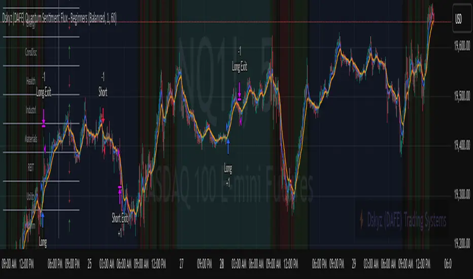
Dskyz (DAFE) Quantum Sentiment Flux - Beginners Dskyz (DAFE) Quantum Sentiment Flux - Beginners:
Welcome to the Dskyz (DAFE) Quantum Sentiment Flux - Beginners , a strategy and concept that’s your ultimate wingman for trading futures like MNQ, NQ, MES, and ES. This gem combines lightning-fast momentum signals, market sentiment smarts, and bulletproof risk management into a system so intuitive, even newbies can trade like pros. With clean DAFE visuals, preset modes for every vibe, and a revamped dashboard that’s basically a market GPS, this strategy makes futures trading feel like a high-octane sci-fi mission.
Built on the Dskyz (DAFE) legacy of Aurora Divergence, the Quantum Sentiment Flux is designed to empower beginners while giving seasoned traders a lean, sentiment-driven edge. It uses fast/slow EMA crossovers for entries, filters trades with VIX, SPX trends, and sector breadth, and keeps your account safe with adaptive stops and cooldowns. Tuned for more action with faster signals and a slick bottom-left dashboard, this updated version is ready to light up your charts and outsmart institutional traps. Let’s dive into why this strat’s a must-have and break down its brilliance.
Why Traders Need This Strategy
Futures markets are a wild ride—fast moves, volatility spikes (like the April 28, 2025 NQ 1k-point drop), and institutional games that can wreck unprepared traders. Beginners often get lost in complex systems or burned by impulsive trades. The Quantum Sentiment Flux is the antidote, offering:
Dead-Simple Setup: Preset modes (Aggressive, Balanced, Conservative) auto-tune signals, risk, and sizing, so you can trade without a quant degree.
Sentiment Superpower: VIX filter, SPX trend, and sector breadth visuals keep you aligned with market health, dodging chop and riding trends.
Ironclad Safety: Tighter ATR-based stops, 2:1 take-profits, and preset cooldowns protect your capital, even in chaotic sessions.
Next-Level Visuals: Green/red entry triangles, vibrant EMAs, a sector breadth background, and a beefed-up dashboard make signals and context pop.
DAFE Swagger: The clean aesthetics, sleek dashboard—ties it to Dskyz’s elite brand, making your charts a work of art.
Traders need this because it’s a plug-and-play system that blends beginner-friendly simplicity with pro-level market awareness. Whether you’re just starting or scalping 5min MNQ, this strat’s your key to trading with confidence and style.
Strategy Components
1. Core Signal Logic (High-Speed Momentum)
The strategy’s engine is a momentum-based system using fast and slow Exponential Moving Averages (EMAs), now tuned for faster, more frequent trades.
How It Works:
Fast/Slow EMAs: Fast EMA (Aggressive: 5, Balanced: 7, Conservative: 9 bars) and slow EMA (12/14/18 bars) track short-term vs. longer-term momentum.
Crossover Signals:
Buy: Fast EMA crosses above slow EMA, and trend_dir = 1 (fast EMA > slow EMA + ATR * strength threshold).
Sell: Fast EMA crosses below slow EMA, and trend_dir = -1 (fast EMA < slow EMA - ATR * strength threshold).
Strength Filter: ma_strength = fast EMA - slow EMA must exceed an ATR-scaled threshold (Aggressive: 0.15, Balanced: 0.18, Conservative: 0.25) for robust signals.
Trend Direction: trend_dir confirms momentum, filtering out weak crossovers in choppy markets.
Evolution:
Faster EMAs (down from 7–10/21–50) catch short-term trends, perfect for active futures markets.
Lower strength thresholds (0.15–0.25 vs. 0.3–0.5) make signals more sensitive, boosting trade frequency without sacrificing quality.
Preset tuning ensures beginners get optimized settings, while pros can tweak via mode selection.
2. Market Sentiment Filters
The strategy leans hard into market sentiment with a VIX filter, SPX trend analysis, and sector breadth visuals, keeping trades aligned with the big picture.
VIX Filter:
Logic: Blocks long entries if VIX > threshold (default: 20, can_long = vix_close < vix_limit). Shorts are always allowed (can_short = true).
Impact: Prevents longs during high-fear markets (e.g., VIX spikes in crashes), while allowing shorts to capitalize on downturns.
SPX Trend Filter:
Logic: Compares S&P 500 (SPX) close to its SMA (Aggressive: 5, Balanced: 8, Conservative: 12 bars). spx_trend = 1 (UP) if close > SMA, -1 (DOWN) if < SMA, 0 (FLAT) if neutral.
Impact: Provides dashboard context, encouraging trades that align with market direction (e.g., longs in UP trend).
Sector Breadth (Visual):
Logic: Tracks 10 sector ETFs (XLK, XLF, XLE, etc.) vs. their SMAs (same lengths as SPX). Each sector scores +1 (bullish), -1 (bearish), or 0 (neutral), summed as breadth (-10 to +10).
Display: Green background if breadth > 4, red if breadth < -4, else neutral. Dashboard shows sector trends (↑/↓/-).
Impact: Faster SMA lengths make breadth more responsive, reflecting sector rotations (e.g., tech surging, energy lagging).
Why It’s Brilliant:
- VIX filter adds pro-level volatility awareness, saving beginners from panic-driven losses.
- SPX and sector breadth give a 360° view of market health, boosting signal confidence (e.g., green BG + buy signal = high-probability trade).
- Shorter SMAs make sentiment visuals react faster, perfect for 5min charts.
3. Risk Management
The risk controls are a fortress, now tighter and more dynamic to support frequent trading while keeping accounts safe.
Preset-Based Risk:
Aggressive: Fast EMAs (5/12), tight stops (1.1x ATR), 1-bar cooldown. High trade frequency, higher risk.
Balanced: EMAs (7/14), 1.2x ATR stops, 1-bar cooldown. Versatile for most traders.
Conservative: EMAs (9/18), 1.3x ATR stops, 2-bar cooldown. Safer, fewer trades.
Impact: Auto-scales risk to match style, making it foolproof for beginners.
Adaptive Stops and Take-Profits:
Logic: Stops = entry ± ATR * atr_mult (1.1–1.3x, down from 1.2–2.0x). Take-profits = entry ± ATR * take_mult (2x stop distance, 2:1 reward/risk). Longs: stop below entry, TP above; shorts: vice versa.
Impact: Tighter stops increase trade turnover while maintaining solid risk/reward, adapting to volatility.
Trade Cooldown:
Logic: Preset-driven (Aggressive/Balanced: 1 bar, Conservative: 2 bars vs. old user-input 2). Ensures bar_index - last_trade_bar >= cooldown.
Impact: Faster cooldowns (especially Aggressive/Balanced) allow more trades, balanced by VIX and strength filters.
Contract Sizing:
Logic: User sets contracts (default: 1, max: 10), no preset cap (unlike old 7/5/3 suggestion).
Impact: Flexible but risks over-leverage; beginners should stick to low contracts.
Built To Be Reliable and Consistent:
- Tighter stops and faster cooldowns make it a high-octane system without blowing up accounts.
- Preset-driven risk removes guesswork, letting newbies trade confidently.
- 2:1 TPs ensure profitable trades outweigh losses, even in volatile sessions like April 27, 2025 ES slippage.
4. Trade Entry and Exit Logic
The entry/exit rules are simple yet razor-sharp, now with VIX filtering and faster signals:
Entry Conditions:
Long Entry: buy_signal (fast EMA crosses above slow EMA, trend_dir = 1), no position (strategy.position_size = 0), cooldown passed (can_trade), and VIX < 20 (can_long). Enters with user-defined contracts.
Short Entry: sell_signal (fast EMA crosses below slow EMA, trend_dir = -1), no position, cooldown passed, can_short (always true).
Logic: Tracks last_entry_bar for visuals, last_trade_bar for cooldowns.
Exit Conditions:
Stop-Loss/Take-Profit: ATR-based stops (1.1–1.3x) and TPs (2x stop distance). Longs exit if price hits stop (below) or TP (above); shorts vice versa.
No Other Exits: Keeps it straightforward, relying on stops/TPs.
5. DAFE Visuals
The visuals are pure DAFE magic, blending clean function with informative metrics utilized by professionals, now enhanced by faster signals and a responsive breadth background:
EMA Plots:
Display: Fast EMA (blue, 2px), slow EMA (orange, 2px), using faster lengths (5–9/12–18).
Purpose: Highlights momentum shifts, with crossovers signaling entries.
Sector Breadth Background:
Display: Green (90% transparent) if breadth > 4, red (90%) if breadth < -4, else neutral.
Purpose: Faster breadth_sma_len (5–12 vs. 10–50) reflects sector shifts in real-time, reinforcing signal strength.
- Visuals are intuitive, turning complex signals into clear buy/sell cues.
- Faster breadth background reacts to market rotations (e.g., tech vs. energy), giving a pro-level edge.
6. Sector Breadth Dashboard
The new bottom-left dashboard is a game-changer, a 3x16 table (black/gray theme) that’s your market command center:
Metrics:
VIX: Current VIX (red if > 20, gray if not).
SPX: Trend as “UP” (green), “DOWN” (red), or “FLAT” (gray).
Trade Longs: “OK” (green) if VIX < 20, “BLOCK” (red) if not.
Sector Breadth: 10 sectors (Tech, Financial, etc.) with trend arrows (↑ green, ↓ red, - gray).
Placeholder Row: Empty for future metrics (e.g., ATR, breadth score).
Purpose: Consolidates regime, volatility, market trend, and sector data, making decisions a breeze.
- VIX and SPX metrics add context, helping beginners avoid bad trades (e.g., no longs if “BLOCK”).
Sector arrows show market health at a glance, like a cheat code for sentiment.
Key Features
Beginner-Ready: Preset modes and clear visuals make futures trading a breeze.
Sentiment-Driven: VIX filter, SPX trend, and sector breadth keep you in sync with the market.
High-Frequency: Faster EMAs, tighter stops, and short cooldowns boost trade volume.
Safe and Smart: Adaptive stops/TPs and cooldowns protect capital while maximizing wins.
Visual Mastery: DAFE’s clean flair, EMAs, dashboard—makes trading fun and clear.
Backtestable: Lean code and fixed qty ensure accurate historical testing.
How to Use
Add to Chart: Load on a 5min MNQ/ES chart in TradingView.
Pick Preset: Aggressive (scalping), Balanced (versatile), or Conservative (safe). Balanced is default.
Set Contracts: Default 1, max 10. Stick low for safety.
Check Dashboard: Bottom-left shows preset, VIX, SPX, and sectors. “OK” + green breadth = strong buy.
Backtest: Run in strategy tester to compare modes.
Live Trade: Connect to Tradovate or similar. Watch for slippage (e.g., April 27, 2025 ES issues).
Replay Test: Try April 28, 2025 NQ drop to see VIX filter and stops in action.
Why It’s Brilliant
The Dskyz (DAFE) Quantum Sentiment Flux - Beginners is a masterpiece of simplicity and power. It takes pro-level tools—momentum, VIX, sector breadth—and wraps them in a system anyone can run. Faster signals and tighter stops make it a trading machine, while the VIX filter and dashboard keep you ahead of market chaos. The DAFE visuals and bottom-left command center turn your chart into a futuristic cockpit, guiding you through every trade. For beginners, it’s a safe entry to futures; for pros, it’s a scalping beast with sentiment smarts. This strat doesn’t just trade—it transforms how you see the market.
Final Notes
This is more than a strategy—it’s your launchpad to mastering futures with Dskyz (DAFE) flair. The Quantum Sentiment Flux blends accessibility, speed, and market savvy to help you outsmart the game. Load it, watch those triangles glow, and let’s make the markets your canvas!
Official Statement from Pine Script Team
(see TradingView help docs and forums):
"This warning may appear when you call functions such as ta.sma inside a request.security in a loop. There is no runtime impact. If you need to loop through a dynamic list of tickers, this cannot be avoided in the present version... Values will still be correct. Ignore this warning in such contexts."
(This publishing will most likely be taken down do to some miscellaneous rule about properly displaying charting symbols, or whatever. Once I've identified what part of the publishing they want to pick on, I'll adjust and repost.)
Use it with discipline. Use it with clarity. Trade smarter.
**I will continue to release incredible strategies and indicators until I turn this into a brand or until someone offers me a contract.
Created by Dskyz, powered by DAFE Trading Systems. Trade fast, trade bold.
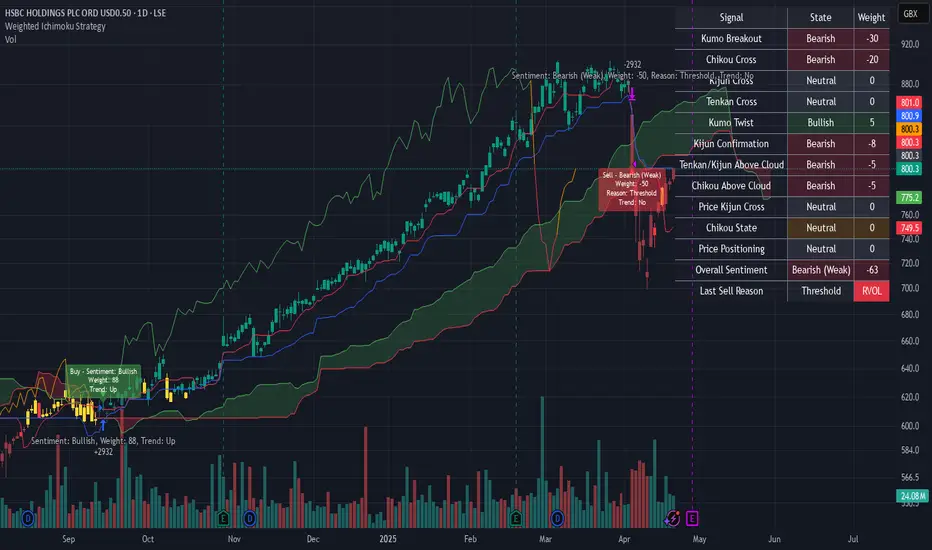
Weighted Ichimoku StrategyLSE:HSBA
The Ichimoku Kinko Hyo indicator is a comprehensive tool that combines multiple signals to identify market trends and potential buying/selling opportunities. My weighted variant of this strategy attempts to assign specific weights to each signal, allowing for a more nuanced and customizable approach to trend identification. The intent is to try and make a more informed trading decision based on the cumulative strength of various signals.
I've tried not to make it a mishmash of this and that + MACD + RSI and on and on; most people have their preferred indicator that focuses on just that that they can use in conjunction.
The signals used can be grouped into two groups the 'Core Ichimoku Signals' & the 'Additional Signals' (at the end you will find the signals and their assigned weights followed by the thresholds where they align).
The Core Ichimoku Signals are the primary signals used in Ichimoku analysis, including Kumo Breakout, Chikou Cross, Kijun Cross, Tenkan Cross, and Kumo Twist.
While the Additional Signals provide further insights and confirmations, such as Kijun Confirmation, Tenkan-Kijun Above Cloud, Chikou Above Cloud, Price-Kijun Cross, Chikou Span Signal, and Price Positioning.
Entries are triggered when the cumulative weight of bullish signals exceeds a specified buy threshold, indicating a strong uptrend or potential trend reversal.
Exits are initiated when the cumulative weight of bearish signals surpasses a specified sell threshold, or when additional conditions such as consolidation patterns or ATR-based targets are met.
There are various exit types that you can choose between, which can be used separately or in conjunction with one another. As an example you might want to exit on a different condition during consolidation periods than during other periods or just use ATR with some other backstop.
They are listed in evaluation order i.e. ATR trumps all, Consolidation exit trumps the regular Kumo sell and so on:
**ATR Sell**: Exits trades based on ATR-based profit targets and stop-losses.
**Consolidation Exit**: Exits trades during consolidation periods to reduce drawdown.
**Sell Below Kumo**: Exits trades when the price is below the Kumo, indicating a potential downtrend.
**Sell Threshold**: Exits trades when the cumulative weight of bearish signals surpasses a specified sell threshold.
There are various 'filters' which are really behavior modifiers:
**Kumo Breakout Filter**: Requires price to close above the Kumo for buy signals (essentially a entry delay).
**Whipsaw Filter**: Ensures trend strength over specified days to reduce false signals.
**Buy Cooldown**: Prevents new entries until half the Kijun period passes after an exit (prevents flapping).
**Chikou Filter**: Delays exits unless the previous close is below the Chikou Span.
**Consolidation Trend Filter**: Prevents consolidation exits if the trend is bullish (rare, but happens).
Then there are some debugging options. Ichimoku periods have some presets (personally I like 8/22/44/22) but are freely configurable, preset to the traditional values for purists.
The list of signals and most thresholds follow, play around with them. Thats all.
Cheers,
**Core Ichimoku Signals**
**Kumo Breakout**
- 30 (Bullish) / -30 (Bearish)
- Indicates a strong trend when the price breaks above (bullish) or below (bearish) the Kumo (cloud). This signal suggests a significant shift in market sentiment.
**Chikou Cross**
- 20 (Bullish) / -20 (Bearish)
- Shows the relationship between the Chikou Span (lagging span) and the current price. A bullish signal occurs when the Chikou Span is above the price, indicating a potential uptrend. Conversely, a bearish signal occurs when the Chikou Span is below the price, suggesting a downtrend.
**Kijun Cross**
- 15 (Bullish) / -15 (Bearish)
- Signals trend changes when the Tenkan-sen (conversion line) crosses above (bullish) or below (bearish) the Kijun-sen (base line). This crossover is often used to identify potential trend reversals.
**Tenkan Cross**
- 10 (Bullish) / -10 (Bearish)
- Indicates short-term trend changes when the price crosses above (bullish) or below (bearish) the Tenkan-sen. This signal helps identify minor trend shifts within the broader trend.
**Kumo Twist**
- 5 (Bullish) / -5 (Bearish)
- Shows changes in the Kumo's direction, indicating potential trend shifts. A bullish Kumo Twist occurs when Senkou Span A crosses above Senkou Span B, and a bearish twist occurs when Senkou Span A crosses below Senkou Span B.
**Additional Signals**
**Kijun Confirmation**
- 8 (Bullish) / -8 (Bearish)
- Confirms the trend based on the price's position relative to the Kijun-sen. A bullish signal occurs when the price is above the Kijun-sen, and a bearish signal occurs when the price is below it.
**Tenkan-Kijun Above Cloud**
- 5 (Bullish) / -5 (Bearish)
- Indicates a strong bullish trend when both the Tenkan-sen and Kijun-sen are above the Kumo. Conversely, a bearish signal occurs when both lines are below the Kumo.
**Chikou Above Cloud**
- 5 (Bullish) / -5 (Bearish)
- Shows the Chikou Span's position relative to the Kumo, indicating trend strength. A bullish signal occurs when the Chikou Span is above the Kumo, and a bearish signal occurs when it is below.
**Price-Kijun Cross**
- 2 (Bullish) / -2 (Bearish)
- Signals short-term trend changes when the price crosses above (bullish) or below (bearish) the Kijun-sen. This signal is similar to the Kijun Cross but focuses on the price's direct interaction with the Kijun-sen.
**Chikou Span Signal**
- 10 (Bullish) / -10 (Bearish)
- Indicates the trend based on the Chikou Span's position relative to past price highs and lows. A bullish signal occurs when the Chikou Span is above the highest high of the past period, and a bearish signal occurs when it is below the lowest low.
**Price Positioning**
- 10 (Bullish) / -10 (Bearish)
- Shows indecision when the price is between the Tenkan-sen and Kijun-sen, indicating a potential consolidation phase. A bullish signal occurs when the price is above both lines, and a bearish signal occurs when the price is below both lines.
**Confidence Level**: Highly Sensitive
- **Buy Threshold**: 50
- **Sell Threshold**: -50
- **Notes / Significance**: ~2–3 signals, very early trend detection. High sensitivity, may capture noise and false signals.
**Confidence Level**: Entry-Level
- **Buy Threshold**: 58
- **Sell Threshold**: -58
- **Notes / Significance**: ~3–4 signals, often Chikou Cross or Kumo Breakout. Very sensitive, risks noise (e.g., false buys in choppy markets).
**Confidence Level**: Entry-Level
- **Buy Threshold**: 60
- **Sell Threshold**: -60
- **Notes / Significance**: ~3–4 signals, Kumo Breakout or Chikou Cross anchors. Entry point for early trends.
**Confidence Level**: Moderate
- **Buy Threshold**: 65
- **Sell Threshold**: -65
- **Notes / Significance**: ~4–5 signals, balances sensitivity and reliability. Suitable for moderate risk tolerance.
**Confidence Level**: Conservative
- **Buy Threshold**: 70
- **Sell Threshold**: -70
- **Notes / Significance**: ~4–5 signals, emphasizes stronger confirmations. Reduces false signals but may miss some opportunities.
**Confidence Level**: Very Conservative
- **Buy Threshold**: 75
- **Sell Threshold**: -75
- **Notes / Significance**: ~5–6 signals, prioritizes high confidence. Minimizes risk but may enter trades late.
**Confidence Level**: High Confidence
- **Buy Threshold**: 80
- **Sell Threshold**: -80
- **Notes / Significance**: ~6–7 signals, very strong confirmations needed. Suitable for cautious traders.
**Confidence Level**: Very High Confidence
- **Buy Threshold**: 85
- **Sell Threshold**: -85
- **Notes / Significance**: ~7–8 signals, extremely high confidence required. Minimizes false signals significantly.
**Confidence Level**: Maximum Confidence
- **Buy Threshold**: 90
- **Sell Threshold**: -90
- **Notes / Significance**: ~8–9 signals, maximum confidence level. Ensures trades are highly reliable but may result in fewer trades.
**Confidence Level**: Ultra Conservative
- **Buy Threshold**: 100
- **Sell Threshold**: -100
- **Notes / Significance**: ~9–10 signals, ultra-high confidence. Trades are extremely reliable but opportunities are rare.
**Confidence Level**: Extreme Confidence
- **Buy Threshold**: 110
- **Sell Threshold**: -110
- **Notes / Significance**: All signals align, extreme confidence. Trades are almost certain but very few opportunities.
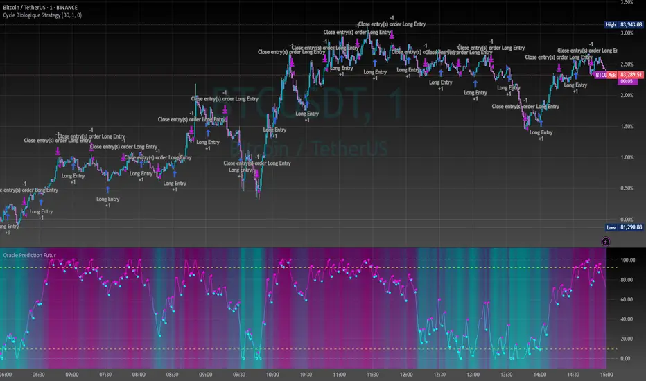
Cycle Biologique Strategy // (\_/)
// ( •.•)
// (")_(")
//@fr33domz
Experimental Research: Cycle Biologique Strategy
Overview
The "Cycle Biologique Strategy" is an experimental trading algorithm designed to leverage periodic cycles in price movements by utilizing a sinusoidal function. This strategy aims to identify potential buy and sell signals based on the behavior of a custom-defined biological cycle.
Key Parameters
Cycle Length: This parameter defines the duration of the cycle, set by default to 30 periods. The user can adjust this value to optimize the strategy for different asset classes or market conditions.
Amplitude: The amplitude of the cycle influences the scale of the sinusoidal wave, allowing for customization in the sensitivity of buy and sell signals.
Offset: The offset parameter introduces phase shifts to the cycle, adjustable within a range of -360 to 360 degrees. This flexibility allows the strategy to align with various market rhythms.
Methodology
The core of the strategy lies in the calculation of a periodic cycle using a sinusoidal function.
Trading Signals
Buy Signal: A buy signal is generated when the cycle value crosses above zero, indicating a potential upward momentum.
Sell Signal: Conversely, a sell signal is triggered when the cycle value crosses below zero, suggesting a potential downtrend.
Execution
The strategy executes trades based on these signals:
Upon receiving a buy signal, the algorithm enters a long position.
When a sell signal occurs, the strategy closes the long position.
Visualization
To enhance user experience, the periodic cycle is plotted visually on the chart in blue, allowing traders to observe the cyclical nature of the strategy and its alignment with market movements.
TheRookAlgoPROThe Rook Algo PRO is an automated strategy that uses ICT dealing ranges to get in sync with potential market trends. It detects the market sentiment and then place a sell or a buy trade in premium/discount or in breakouts with the desired risk management.
Why is useful?
This algorithm is designed to help traders to quickly identify the current state of the market and easily back test their strategy over longs periods of time and different markets its ideal for traders that want to profit on potential expansions and want to avoid consolidations this algo will tell you when the expansion is likely to begin and when is just consolidating and failing moves to avoid trading.
How it works and how it does it?
The Algo detects the current and previous market structure to identify current ranges and ICT dealing ranges that are created when the market takes buyside liquidity and sellside liquidity, it will tell if the market is in a consolidation, expansion, retracement or in a potential turtle soup environment, it will tell if the range is small or big compared to the previous one. Is important to use it in a trending markets because when is ranging the signals lose effectiveness.
This algo is similar to the previously released the Rook algo with the additional features that is an automated strategy that can take trades using filters with the desired risk reward and different entry types and trade management options.
Also this version plots FVGS(fair value gaps) during expansions, and detects consolidations with a box and the mid point or average. Some bars colors are available to help in the identification of the market state. It has the option to show colors of the dealing ranges first detected state.
How to use it?
Start selecting the desired type of entry you want to trade, you can choose to take Discount longs, premium sells, breakouts longs and sells, this first four options are the selected by default. You can enable riskier options like trades without confirmation in premium and discount or turtle soup of the current or previous dealing range. This last ones are ideal for traders looking to enter on a counter trend but has to be used with caution with a higher timeframe reference.
In the picture below we can see a premium sell signal configuration followed by a discount buy signal It display the stop break even level and take profit.
This next image show how the riskier entries work. Because we are not waiting for a confirmation and entering on a counter trend is normal to experience some stop losses because the stop is very tight. Should only be used with a clear Higher timeframe reference as support of the trade idea. This algo has the option to enable standard deviations from the normal stop point to prevent liquidity sweeps. The purple or blue arrows indicate when we are in a potential turtle soup environment.
The algo have a feature called auto-trade enable by default that allow for a reversal of the current trade in case it meets the criteria. And also can take all possible buys or all possible sells that are riskier entries if you just want to see the market sentiment. This is useful when the market is very volatile but is moving not just ranging.
Then we configure the desired trade filters. We have the options to trade only when dealing ranges are in sync for a more secure trend, or we can disable it to take riskier trades like turtle soup trades. We can chose the minimum risk reward to take the trade and the target extension from the current range and the exit type can be when we hit the level or in a retracement that is the default setting. These setting are the most important that determine profitability of the strategy, they has be adjusted depending on the timeframe and market we are trading.
The stop and target levels can also be configured with standard deviations from the current range that way can be adapted to the market volatility.
The Algo allow the user to chose if it want to place break even, or trail the stop. In the picture below we can see it in action. This can work when the trend is very strong if not can lead to multiple reentries or loses.
The last option we can configure is the time where the trades are going to be taken, if we trade usually in the morning then we can just add the morning time by default is set to the morning 730am to 1330pm if you want to trade other times you should change this. Or if we want to enter on the ICT macro times can also be added in a filter. Trade taken with the macro times only enable is visible in the picture below.
Strategy Results
The results are obtained using 2000usd in the MNQ! In the 15minutes timeframe 1 contract per trade. Commission are set to 2USD, slippage to 1tick, the backtesting range is from May 2 2024 to March 2025 for a total of 119 trades, this Strategy default settings are designed to take trades on the daily expansions, trail stop and Break even is activated the exit on profit is on a retracement, and for loses when the stop is hit. The auto-trade option is enable to allow to detect quickly market changes. The strategy give realistic results, makes around 200% of the account in around a year. 1.4 profit factor with around 37% profitable trades. These results can be further improve and adapted to the specific style of trading using the filters.
Remember entries constitute only a small component of a complete winning strategy. Other factors like risk management, position-sizing, trading frequency, trading fees, and many others must also be properly managed to achieve profitability. Past performance doesn’t guarantee future results.
Summary of features
-Easily Identify the current dealing range and market state to avoid consolidations
-Recognize expansions with FVGs and consolidation with shaded boxes
-Recognize turtle soups scenarios to avoid fake out breakout
-Configurable automated trades in premium/discount or breakouts
-Auto-trade option that allow for reversal of the current trade when is no longer valid
-Time filter to allow only entries around the times you trade or on the macro times.
-Risk Reward filter to take the automated trades with visible stop and take profit levels
-Customizable trade management take profit, stop, breakeven level with standard deviations
-Trail stop option to secure profit when price move in your favor
-Option to exit on a close, retracement or reversal after hitting the take profit level
-Option to exit on a close or reversal after hitting stop loss
-Dashboard with instant statistics about the strategy current settings and market sentiment

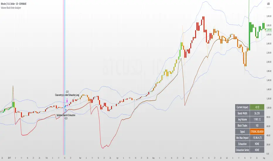
Volume Block Order AnalyzerCore Concept
The Volume Block Order Analyzer is a sophisticated Pine Script strategy designed to detect and analyze institutional money flow through large block trades. It identifies unusually high volume candles and evaluates their directional bias to provide clear visual signals of potential market movements.
How It Works: The Mathematical Model
1. Volume Anomaly Detection
The strategy first identifies "block trades" using a statistical approach:
```
avgVolume = ta.sma(volume, lookbackPeriod)
isHighVolume = volume > avgVolume * volumeThreshold
```
This means a candle must have volume exceeding the recent average by a user-defined multiplier (default 2.0x) to be considered a significant block trade.
2. Directional Impact Calculation
For each block trade identified, its price action determines direction:
- Bullish candle (close > open): Positive impact
- Bearish candle (close < open): Negative impact
The magnitude of impact is proportional to the volume size:
```
volumeWeight = volume / avgVolume // How many times larger than average
blockImpact = (isBullish ? 1.0 : -1.0) * (volumeWeight / 10)
```
This creates a normalized impact score typically ranging from -1.0 to 1.0, scaled by dividing by 10 to prevent excessive values.
3. Cumulative Impact with Time Decay
The key innovation is the cumulative impact calculation with decay:
```
cumulativeImpact := cumulativeImpact * impactDecay + blockImpact
```
This mathematical model has important properties:
- Recent block trades have stronger influence than older ones
- Impact gradually "fades" at rate determined by decay factor (default 0.95)
- Sustained directional pressure accumulates over time
- Opposing pressure gradually counteracts previous momentum
Trading Logic
Signal Generation
The strategy generates trading signals based on momentum shifts in institutional order flow:
1. Long Entry Signal: When cumulative impact crosses from negative to positive
```
if ta.crossover(cumulativeImpact, 0)
strategy.entry("Long", strategy.long)
```
*Logic: Institutional buying pressure has overcome selling pressure, indicating potential upward movement*
2. Short Entry Signal: When cumulative impact crosses from positive to negative
```
if ta.crossunder(cumulativeImpact, 0)
strategy.entry("Short", strategy.short)
```
*Logic: Institutional selling pressure has overcome buying pressure, indicating potential downward movement*
3. Exit Logic: Positions are closed when the cumulative impact moves against the position
```
if cumulativeImpact < 0
strategy.close("Long")
```
*Logic: The original signal is no longer valid as institutional flow has reversed*
Visual Interpretation System
The strategy employs multiple visualization techniques:
1. Color Gradient Bar System:
- Deep green: Strong buying pressure (impact > 0.5)
- Light green: Moderate buying pressure (0.1 < impact ≤ 0.5)
- Yellow-green: Mild buying pressure (0 < impact ≤ 0.1)
- Yellow: Neutral (impact = 0)
- Yellow-orange: Mild selling pressure (-0.1 < impact ≤ 0)
- Orange: Moderate selling pressure (-0.5 < impact ≤ -0.1)
- Red: Strong selling pressure (impact ≤ -0.5)
2. Dynamic Impact Line:
- Plots the cumulative impact as a line
- Line color shifts with impact value
- Line movement shows momentum and trend strength
3. Block Trade Labels:
- Marks significant block trades directly on the chart
- Shows direction and volume amount
- Helps identify key moments of institutional activity
4. Information Dashboard:
- Current impact value and signal direction
- Average volume benchmark
- Count of significant block trades
- Min/Max impact range
Benefits and Use Cases
This strategy provides several advantages:
1. Institutional Flow Detection: Identifies where large players are positioning themselves
2. Early Trend Identification: Often detects institutional accumulation/distribution before major price movements
3. Market Context Enhancement: Provides deeper insight than simple price action alone
4. Objective Decision Framework: Quantifies what might otherwise be subjective observations
5. Adaptive to Market Conditions: Works across different timeframes and instruments by using relative volume rather than absolute thresholds
Customization Options
The strategy allows users to fine-tune its behavior:
- Volume Threshold: How unusual a volume spike must be to qualify
- Lookback Period: How far back to measure average volume
- Impact Decay Factor: How quickly older trades lose influence
- Visual Settings: Labels and line width customization
This sophisticated yet intuitive strategy provides traders with a window into institutional activity, helping identify potential trend changes before they become obvious in price action alone.
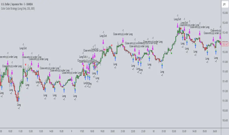
Color Code Overlay StrategyColor Code Overlay Strategy
This strategy utilizes a custom color-coded overlay to provide accurate buy and sell signals based on dynamic color changes of the candles. The indicator works by calculating a color shift between bullish (green) and bearish (red) candles, with the color change logic driven by both price movement and volatility.
How the Color Change is Calculated:
The color change is determined by comparing the closing price relative to the opening price of each candle, as is typical with a traditional bullish or bearish candle. However, to make this strategy more adaptive to market conditions, the color change is further refined by incorporating the Average True Range (ATR).
Volatility Adjusted Color Shift: The strategy calculates a dynamic threshold based on the ATR value, which represents market volatility. If the price movement between the open and close of the candle exceeds a specific percentage of the ATR, the color of the candle shifts from red (bearish) to green (bullish) or vice versa.
Threshold Calculation: A fixed percentage (e.g., 1%) of the ATR range is used to define the minimum price movement required for a color change. This ensures that only significant price movements, adjusted for volatility, trigger the color shift. The larger the ATR (higher volatility), the greater the price movement required to cause a change in color.
Bullish to Bearish (Green to Red): When the candle closes lower than the open, and the price movement exceeds the dynamic threshold based on ATR, the candle color changes from green to red, signaling a potential bearish reversal.
Bearish to Bullish (Red to Green): When the candle closes higher than the open, and the price movement exceeds the ATR-based threshold, the candle color shifts from red to green, signaling a potential bullish reversal.
Key Features:
Dynamic Color Change: The strategy identifies key color changes from bullish to bearish (green to red) and from bearish to bullish (red to green) based on specific thresholds in candle size.
Customizable Timeframe: You can specify a custom trading window to restrict the strategy’s actions to specific hours of the day.
Stop Loss and Take Profit: The strategy incorporates risk management features, allowing you to set a stop loss and take profit based on the price in pips.
Flexible Trade Types: Choose between "Both" (long and short), "Long Only," or "Short Only" trading options to suit your preferred trading style.
Visual Alerts: Receive visual alerts with arrows when color changes occur, signaling potential trade opportunities. Green arrows indicate a bullish shift, while red arrows show a bearish shift.
This strategy is ideal for traders who prefer a color-coded overlay to easily visualize price action and make informed decisions based on bullish or bearish trends. Whether you’re looking for quick, short-term opportunities or analyzing market reversals, this strategy offers an intuitive approach to identifying trade signals.
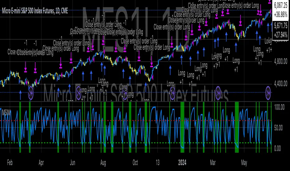
Macro-Sentiment Index Model (MSIM)Macro-Sentiment Index Model (MSIM) is a comprehensive trading strategy developed to analyze and interpret the broader macroeconomic and market sentiment. The strategy integrates various quantitative signals, including market volatility, trading volume, market breadth, and economic indicators, to assess the prevailing mood in the financial markets. This sentiment analysis is then used to guide trading decisions, helping identify optimal entry and exit points based on underlying market conditions. The model is specifically designed to capture the shifts in investor sentiment, which have been shown to significantly influence market behavior (Fleming et al., 2001).
The MSIM utilizes a multi-faceted approach to measure sentiment. Drawing from the theory that macroeconomic variables can influence financial markets (Stock & Watson, 2002), the strategy incorporates market volatility (VIX), volume measures, and long-term market trends. These indicators help form a robust view of the market’s risk appetite and potential for price movement. For instance, high volatility often signals increased market uncertainty (Bollerslev, 1986), while volume-based indicators provide insights into investor conviction (Chen, 1991).
Additionally, the model incorporates macroeconomic proxies like GDP growth, interest rates, and unemployment data, leveraging the findings of macroeconomic studies that indicate a direct correlation between these factors and market performance (Hamilton, 1994). By normalizing these economic indicators, the model provides a standardized sentiment score that reflects the aggregated impact of these factors on the market’s outlook.
The MSIM aims to exploit market inefficiencies by responding to shifts in sentiment before they manifest in price movements. Studies have shown that sentiment indicators, such as the Advance-Decline Line and the Stock-Bond Ratio, can be predictive of future price movements (Neely, 2010). The model integrates these indicators into a single composite sentiment score, which is then filtered through momentum signals to refine entry points. This approach is grounded in behavioral finance theory, which suggests that investor sentiment plays a crucial role in driving asset prices, sometimes beyond the reach of fundamental data alone (Shiller, 2000).
The strategy is designed to identify long opportunities when sentiment is particularly favorable, with a focus on minimizing risk during adverse conditions. By analyzing market trends alongside macroeconomic signals, the MSIM helps traders stay aligned with the prevailing market forces.
References:
• Bollerslev, T. (1986). Generalized autoregressive conditional heteroskedasticity. Journal of Econometrics, 31(3), 307-327.
• Chen, S. S. (1991). The determinants of stock market liquidity. Journal of Financial and Quantitative Analysis, 26(3), 283-305.
• Fleming, M. J., Kirby, C. W., & Ostdiek, B. (2001). The economic value of volatility timing. Journal of Financial and Quantitative Analysis, 36(1), 113-134.
• Hamilton, J. D. (1994). Time series analysis. Princeton University Press.
• Neely, C. J. (2010). The behavior of exchange rates: A survey of recent empirical literature. International Finance Discussion Papers, 981.
• Shiller, R. J. (2000). Irrational Exuberance. Princeton University Press.
• Stock, J. H., & Watson, M. W. (2002). Macroeconomic forecasting using diffusion indexes. Journal of Business & Economic Statistics, 20(2), 147-162.
Candle Emotion Index (CEI) StrategyThe Candle Emotion Index (CEI) Strategy is an innovative sentiment-based trading approach designed to help traders identify and capitalize on market psychology. By analyzing candlestick patterns and combining them into a unified metric, the CEI Strategy provides clear entry and exit signals while dynamically managing risk. This strategy is ideal for traders looking to leverage market sentiment to identify high-probability trading opportunities.
How It Works
The CEI Strategy is built around three core oscillators that reflect key emotional states in the market:
Indecision Oscillator . Measures market uncertainty using patterns like Doji and Spinning Tops. High values indicate hesitation, signaling potential turning points.
Fear Oscillator . Tracks bearish sentiment through patterns like Shooting Star, Hanging Man, and Bearish Engulfing. Helps identify moments of intense selling pressure.
Greed Oscillator . Detects bullish sentiment using patterns like Marubozu, Hammer, Bullish Engulfing, and Three White Soldiers. Highlights periods of strong buying interest.
These oscillators are averaged into the Candle Emotion Index (CEI):
CEI = (Indecision + Fear + Greed) / 3
This single value quantifies overall market sentiment and drives the strategy’s trading decisions.
Key Features
Sentiment-Based Trading Signals . Long Entry: Triggered when the CEI crosses above a lower threshold (e.g., 0.1), indicating increasing bullish sentiment. Short Entry: Triggered when the CEI crosses above a higher threshold (e.g., 0.2), signaling rising bearish sentiment.
Volume Confirmation . Trades are validated only if volume exceeds a user-defined multiplier of the average volume over the lookback period. This ensures entries are backed by significant market activity.
Break-Even Recovery Mechanism . If a trade moves into a loss, the strategy attempts to recover to break-even instead of immediately exiting at a loss. This feature provides flexibility, allowing the market to recover while maintaining disciplined risk management.
Dynamic Risk Management . Maximum Holding Period: Trades are closed after a user-defined number of candles to avoid overexposure to prolonged uncertainty. Profit-Taking Conditions: Positions are exited when favorable price moves are confirmed by increased volume, locking in gains. Loss Threshold: Trades are exited early if the price moves unfavorably beyond a set percentage of the entry price, limiting potential losses.
Cooldown Period . After a trade is closed, a cooldown period prevents immediate re-entry, reducing overtrading and improving signal quality.
Why Use This Strategy?
The CEI Strategy combines advanced sentiment analysis with robust trade management, making it a powerful tool for traders seeking to understand market psychology and identify high-probability setups. Its unique features, such as the break-even recovery mechanism and volume confirmation, add an extra layer of discipline and reliability to trading decisions.
Best Practices
Combine with Other Indicators . Use trend-following tools (e.g., moving averages, ADX) and momentum oscillators (e.g., RSI, MACD) to confirm signals.
Align with Key Levels . Incorporate support and resistance levels for refined entries and exits.
Multi-Market Compatibility . Apply this strategy to forex, crypto, stocks, or any asset class with strong volume and price action.

Dynamic Ticks Oscillator Model (DTOM)The Dynamic Ticks Oscillator Model (DTOM) is a systematic trading approach grounded in momentum and volatility analysis, designed to exploit behavioral inefficiencies in the equity markets. It focuses on the NYSE Down Ticks, a metric reflecting the cumulative number of stocks trading at a lower price than their previous trade. As a proxy for market sentiment and selling pressure, this indicator is particularly useful in identifying shifts in investor behavior during periods of heightened uncertainty or volatility (Jegadeesh & Titman, 1993).
Theoretical Basis
The DTOM builds on established principles of momentum and mean reversion in financial markets. Momentum strategies, which seek to capitalize on the persistence of price trends, have been shown to deliver significant returns in various asset classes (Carhart, 1997). However, these strategies are also susceptible to periods of drawdown due to sudden reversals. By incorporating volatility as a dynamic component, DTOM adapts to changing market conditions, addressing one of the primary challenges of traditional momentum models (Barroso & Santa-Clara, 2015).
Sentiment and Volatility as Core Drivers
The NYSE Down Ticks serve as a proxy for short-term negative sentiment. Sudden increases in Down Ticks often signal panic-driven selling, creating potential opportunities for mean reversion. Behavioral finance studies suggest that investor overreaction to negative news can lead to temporary mispricings, which systematic strategies can exploit (De Bondt & Thaler, 1985). By incorporating a rate-of-change (ROC) oscillator into the model, DTOM tracks the momentum of Down Ticks over a specified lookback period, identifying periods of extreme sentiment.
In addition, the strategy dynamically adjusts entry and exit thresholds based on recent volatility. Research indicates that incorporating volatility into momentum strategies can enhance risk-adjusted returns by improving adaptability to market conditions (Moskowitz, Ooi, & Pedersen, 2012). DTOM uses standard deviations of the ROC as a measure of volatility, allowing thresholds to contract during calm markets and expand during turbulent ones. This approach helps mitigate false signals and aligns with findings that volatility scaling can improve strategy robustness (Barroso & Santa-Clara, 2015).
Practical Implications
The DTOM framework is particularly well-suited for systematic traders seeking to exploit behavioral inefficiencies while maintaining adaptability to varying market environments. By leveraging sentiment metrics such as the NYSE Down Ticks and combining them with a volatility-adjusted momentum oscillator, the strategy addresses key limitations of traditional trend-following models, such as their lagging nature and susceptibility to reversals in volatile conditions.
References
• Barroso, P., & Santa-Clara, P. (2015). Momentum Has Its Moments. Journal of Financial Economics, 116(1), 111–120.
• Carhart, M. M. (1997). On Persistence in Mutual Fund Performance. The Journal of Finance, 52(1), 57–82.
• De Bondt, W. F., & Thaler, R. (1985). Does the Stock Market Overreact? The Journal of Finance, 40(3), 793–805.
• Jegadeesh, N., & Titman, S. (1993). Returns to Buying Winners and Selling Losers: Implications for Stock Market Efficiency. The Journal of Finance, 48(1), 65–91.
• Moskowitz, T. J., Ooi, Y. H., & Pedersen, L. H. (2012). Time Series Momentum. Journal of Financial Economics, 104(2), 228–250.

Stronger V4.0 - Optimized Trading Strategy
Name: Stronger V4.0 - Optimized Trading Strategy
Introduction:
Stronger V4.0 is a structured trading strategy designed to identify and act on market breakout and reversal opportunities. By employing advanced filtering tools such as RSI (Relative Strength Index), MACD (Moving Average Convergence Divergence), and Bollinger Bands, this strategy aims to reduce market noise and provide reliable trading signals.
The strategy dynamically adapts to changing market conditions, focusing on delivering high-quality signals rather than frequent ones. This allows traders to approach markets with more confidence and clarity.
How the Strategy Works and Key Features:
How Stronger V4.0 Works:
Stronger V4.0 combines advanced technical indicators and custom logic to identify optimal entry and exit points in the market. By dynamically integrating filters like RSI, MACD, and Bollinger Bands, the strategy adjusts to market conditions and minimizes noise to deliver high-quality signals.
Key Features:
Dynamic Price Analysis:
Tracks price movements within specific periods to detect breakout and reversal opportunities.
Advanced Filtering Mechanisms:
RSI Filter: Avoids trades in overbought/oversold market conditions.
MACD Filter: Confirms market momentum and trend direction.
Bollinger Bands: Adapts thresholds based on market volatility.
Risk Management:
Limits trade risk to sustainable levels to preserve equity.
Encourages consistent growth by maintaining a maximum risk per trade.
Customizable Parameters:
Users can toggle long or short trades and adjust filter settings to match their trading preferences.
Minimalist Display:
Focuses on essential signals only, ensuring a clean and easy-to-read chart layout.
Market Breakout Identification:
One of Stronger V4.0's core functionalities is identifying significant breakout points. These breakout points are calculated based on dynamic price movements and market momentum.
Key moments are highlighted when the price exits a consolidation phase and transitions into a new trend. These points represent strong market opportunities, offering actionable insights for traders.
Using adjustable period settings, the strategy enables traders to tailor the analysis to their preferred timeframe and trading style. By eliminating market noise, Stronger V4.0 helps traders focus on high-probability setups and make informed decisions during volatile conditions.
Why Stronger V4.0 Stands Out:
Adaptive Filters:
Dynamically integrates RSI, MACD, and Bollinger Bands to reduce noise and highlight high-probability setups.
Precision Execution:
Focuses on executing trades at optimal moments, ensuring a balance between sustainability and profitability.
Rigorous Testing:
Extensively backtested under realistic market conditions for consistent performance.
Tailored and Exclusive:
Designed for traders seeking a balance between quality and adaptability.
Risk Disclaimer:
Stronger V4.0 has been backtested under various market conditions; however, past performance does not guarantee future results. The strategy is provided as-is, and traders are encouraged to test it thoroughly and apply appropriate risk management measures. Always trade responsibly.

TheHorsyAlgoPROThe Horsy algo is an automated strategy that uses any minute Higher timeframe range as reference and search for a purge of liquidity on the HTF high or low where buyside or sell side liquidity is, the algo only search this at specific desired times that can be configured according to the time you usually trade, the strategy is known as Turtle soup purge and reverse or lately as CRT.
Why is useful?
The purpose of this Algorithm is to help turtle soup traders to quickly identify when the market is likely to reverse the algo evaluates if the opportunity is worth it, base on risk reward and other desired filters. Also this strategy can help to quickly backtest the trader strategy it can be configured in different timeframes and adapt to the trader personality, they can easily see the results and statistics and notice if its profitable or not.
This algo is useful for intraday traders looking for a purge and reverse at a key times and at key HTF price levels this only looks the previous HTF highs and lows but is important to also monitor Order blocks, FVGs, gaps, or wicks to have the best results.
How it works and how it does it?
The Horsy algo simply Jumps from one type of liquidity to another one buyside to sell side or vice versa. In order for the algo to trigger an entry it has to meet these conditions
1. Take HTF liquidity, trade above a HTF high or below a HTF low in the selected time window
2. Make a change in the state of delivery with a close below the previous candle low for shorts and close above previous candle high for longs.
3. Allow for a reasonable risk reward, it will use the highest high for shorts and the lowest low for longs. The default take profit is the opposite side of the range.
4. Validate others user filters this include enter only trades aligned with the HTF bias, or trades aligned with the LTF bias or booth. The algo have the option to enter only premium and discount entries. And finally, an option to allow for different contract sizes depending of the maximum percent of the account we want to risk default is 1%. For this last option is important to check the initial balance and leverage are configured correctly, is disable by default because it requires more capital to perform well.
We can see the algo performing in the picture below with a short trade, notice there are some white lines, they are the high or the low of HTF candle that start generating inside candles in the HTF meaning a possible consolidation. The algo plots the HTF ranges in a shaded boxes as you can see below
The HTF bias as you can see in the picture is calculated based on the last close of the HTF meaning close above previous HTF high is bullish close below previous HTF low is bearish. This HTF bias level is also the last HTF mid-price or 50%. By default, this line is enabled.
The LTF bias is calculated based on the range created from the expansion outside the previous HTF range is also the mid-price. If the LTF close above previous HTF high is bullish and if the LTF close below previous HTF low is bearish. By default this LTF bias line is disable.
This strategy includes an original and personal developed code that uses dealing ranges to recognize if the market is expanding, retracing, reversing or consolidating. This allow the algo to exit the position when it detects a retracement or at the end of the expansion. This is the default exit type.
You can monitor the previous dealing ranges created in history with an option than can be enable, by default is disable, this ranges are created after price takes buyside and then sell side or vice versa. So this dealing ranges can be useful also to identify minor pools of liquidity and premium and discount in the lower timeframe.
The picture below is a long example, the exit in this case is just at the high of the range. The normal take profit is in a blue line for longs.
How to use it?
First select the desired HTF timeframe recommended is from 30min to 240min then you setup the chart on the lower timeframe you want to trade recommended is from 1min to 15min to enter. By default This strategy is designed to work for intraday during key times when price take stops and then moves quickly away from them. You can select as much as 6 different times or just one. After you select the desired time window where the algo will look for the purge and reverse, They are highlighted in the candles that change colors excluding the gray ones that indicates consolidation.
Then the Algo allow to performs several additional filters in the entries you can select if you want to trade only longs or shorts trades, you can select when to move the stop loss to Break even. In deviations of the risk or you can just select to remove risk when price hits the 50% of previous HTF range.
You can select the minimum desired risk reward of the trade before is allow to be taken. Once is configured correctly the algo should trigger signals with a triangle up or down plus the strategy entry.
At the beginning of the picture there are some blue lines in the HTF high low and close, this is to easily identify that the market is in the Asia session, the time can be configured by the user, these lines are normally gray.
On the right top of the screen you can see some statistics about the strategy how many trades it took, ARR is an approximated value of the accumulated total risk reward of all the trades when they get closed in the simulation.
Profit factor and percent profitable are also shown should be green it means that the strategy makes money over time. But apart from that is important to notice how it makes money it is stable over time? it is a roller coaster? that why I Include this other measurements MxcsTps is the maximum consecutives take profits and Mxcsls is the maximum consecutive stop losses it takes, the slash number after it is the consecutive Break evens. So this way you know what to expect and what is normal in the strategy.
The algo shows all the times the stop loss, take profit and break even level if enable in the colored red lines for short and blue lines for longs. You can also select how price will manage the profit or stoploss point meaning that you can choose to wait for the candle to close to invalidate your idea or to take profit. This is good to avoid liquidity sweeps but can also lead to mayor loses if the idea is wrong. The default setting is to close the trade when price takes the high or low where the stoploss is, the take profit is taken after a retracement to allow to profit on expansions. You can select also to exit on a reversal if you want to ride all the move. This last option has to be used with caution because sometimes price just retrace or reverse very fast decreasing the trade profit and overall strategy performance.
The algo have the option to use standard deviation from the normal risk if you prefer to prevent liquidity sweeps near the stop level this make wider stops but can lead to increased loses so it has to be used carefully.
Below is a picture that show the entry stop and take profit levels with an exit on a retracement activated.
Strategy Results
The backtesting results are obtained simulating a 2000usd account in the Micro Nasdaq using 1 contract per trade. Commission are set to 2usd per contract, slippage to 1tick. You can see in list of trades we are not risking more than 1 % percent of the account. The backtested range is from august to November 2024. This strategy doesn’t generate too much trades because of the time filters and conditions that has to be meet to take an entry but you can see the results of the last 4months with the available data that are around 32 trades.
The default settings for this strategy is HTF as 240min designed to work on a LTF 5min chart, the default purge times are 245-300, 745-800, 845-900, 1045-1100 and 1245-1300 UTC-4, the algo will look for shorts or longs, with a minimum risk reward of 2.0. With an additional filter of the HTFBias. The take profit is by default taken on the first retracement after hitting the target. The default settings are optimized to work on the Nasdaq or Spy, but can also perform well in other assets with the correct adjustments.
Remember entries constitute only a small component of a complete winning strategy. Other factors like risk management, position-sizing, trading frequency, trading fees, and many others must also be properly managed to achieve profitability. Past performance doesn’t guarantee future results. To really take advantage of this strategy you have to study turtle soup and the HTF key levels use this only as a confirmation that your overall idea will play out and use it to backtest your model.
Summary of features
·Adaptable strategy to different HTF timeframes from 1-1440min
· Select up to 6 different purge time windows UTC-4, UTC-5
· Choose desired Risk Reward per trade
· Easily see the HTF high low close and 50% key levels in the LTF
· Identify HTF consolidations that generate key major liquidity pools
· HTF/LTF bias filters to trade in favor of the big trend or in sync
· Shaded boxes that indicate if the market is bullish, bearish or consolidating
· See the current midpoint of the last expansion move
· Optimal trade entry filter to trade only in a discount or premium
· Customizable trade management take profit, stop, breakeven level
· Option to exit on a close, retracement or reversal after hitting the take profit level
· Option to exit on a close or reversal after hitting stop loss
· Configurable breakeven point with standard deviations or at 50% of the HTF
· Calculate different contract sizes depending of a percentage of the initial balance
· Standard deviations from normal risk can be used to prevent liquidity sweeps
· See dealing ranges history to check minor pools of liquidity and premium or discount
· Dashboard with instant statistics about the strategy current settings

Max Pain StrategyThe Max Pain Strategy uses a combination of volume and price movement thresholds to identify potential "pain zones" in the market. A "pain zone" is considered when the volume exceeds a certain multiple of its average over a defined lookback period, and the price movement exceeds a predefined percentage relative to the price at the beginning of the lookback period.
Here’s how the strategy functions step-by-step:
Inputs:
length: Defines the lookback period used to calculate the moving average of volume and the price change over that period.
volMultiplier: Sets a threshold multiplier for the volume; if the volume exceeds the average volume multiplied by this factor, it triggers the condition for a potential "pain zone."
priceMultiplier: Sets a threshold for the minimum percentage price change that is required for a "pain zone" condition.
Calculations:
averageVolume: The simple moving average (SMA) of volume over the specified lookback period.
priceChange: The absolute difference in price between the current bar's close and the close from the lookback period (length).
Pain Zone Condition:
The condition for entering a position is triggered if both the volume is higher than the average volume by the volMultiplier and the price change exceeds the price at the length-period ago by the priceMultiplier. This is an indication of significant market activity that could result in a price move.
Position Entry:
A long position is entered when the "pain zone" condition is met.
Exit Strategy:
The position is closed after the specified holdPeriods, which defines how many periods the position will be held after being entered.
Visualization:
A small triangle is plotted on the chart where the "pain zone" condition is met.
The background color changes to a semi-transparent red when the "pain zone" is active.
Scientific Explanation of the Components
Volume Analysis and Price Movement: These are two critical factors in trading strategies. Volume often serves as an indicator of market strength (or weakness), and price movement is a direct reflection of market sentiment. Higher volume with significant price movement may suggest that the market is entering a phase of increased volatility or trend formation, which the strategy aims to exploit.
Volume analysis: The study of volume as an indicator of market participation, with increased volume often signaling stronger trends (Murphy, J. J., Technical Analysis of the Financial Markets).
Price movement thresholds: A large price change over a short period may be interpreted as a breakout or a potential reversal point, aligning with volatility and liquidity analysis (Schwager, J. D., Market Wizards).
Repainting Check: This strategy does not involve any repainting because it is based on current and past data, and there is no reference to future values in the decision-making process. However, any strategy that uses lagging indicators or conditions based on historical bars, like close , is inherently a lagging strategy and might not predict real-time price action accurately until after the fact.
Risk Management: The position hold duration is predefined, which adds an element of time-based risk control. This duration ensures that the strategy does not hold a position indefinitely, which could expose it to unnecessary risk.
Potential Issues and Considerations
Repainting:
The strategy does not utilize future data or conditions that depend on future bars, so it does not inherently suffer from repainting issues.
However, since the strategy relies on volume and price change over a set lookback period, the decision to enter or exit a trade is only made after the data for the current bar is complete, meaning the trade decisions are somewhat delayed, which could be seen as a lagging feature rather than a repainting one.
Lagging Nature:
As with many technical analysis-based strategies, this one is based on past data (moving averages, price changes), meaning it reacts to market movements after they have already occurred, rather than predicting future price actions.
Overfitting Risk:
With parameters like the lookback period and multipliers being user-adjustable, there is a risk of overfitting to historical data. Adjusting parameters too much based on past performance can lead to poor out-of-sample results (Gauthier, P., Practical Quantitative Finance).
Conclusion
The Max Pain Strategy is a simple approach to identifying potential market entries based on volume spikes and significant price changes. It avoids repainting by relying solely on historical and current bar data, but it is inherently a lagging strategy that reacts to price and volume patterns after they have occurred. Therefore, the strategy can be effective in trending markets but may struggle in highly volatile, sideways markets.

Global Index Spread RSI StrategyThis strategy leverages the relative strength index (RSI) to monitor the price spread between a global benchmark index (such as AMEX) and the currently opened asset in the chart window. By calculating the spread between these two, the strategy uses RSI to identify oversold and overbought conditions to trigger buy and sell signals.
Key Components:
Global Benchmark Index: The strategy compares the current asset with a predefined global index (e.g., AMEX) to measure relative performance. The choice of a global benchmark allows the trader to analyze the current asset's movement in the context of broader market trends.
Spread Calculation:
The spread is calculated as the percentage difference between the current asset's closing price and the global benchmark index's closing price:
Spread=Current Asset Close−Global Index CloseGlobal Index Close×100
Spread=Global Index CloseCurrent Asset Close−Global Index Close×100
This metric provides a measure of how the current asset is performing relative to the global index. A positive spread indicates the asset is outperforming the benchmark, while a negative spread signals underperformance.
RSI of the Spread: The RSI is then calculated on the spread values. The RSI is a momentum oscillator that ranges from 0 to 100 and is commonly used to identify overbought or oversold conditions in asset prices. An RSI below 30 is considered oversold, indicating a potential buying opportunity, while an RSI above 70 is overbought, suggesting that the asset may be due for a pullback.
Strategy Logic:
Entry Condition: The strategy enters a long position when the RSI of the spread falls below the oversold threshold (default 30). This suggests that the asset may have been oversold relative to the global benchmark and might be due for a reversal.
Exit Condition: The strategy exits the long position when the RSI of the spread rises above the overbought threshold (default 70), indicating that the asset may have become overbought and a price correction is likely.
Visual Reference:
The RSI of the spread is plotted on the chart for visual reference, making it easier for traders to monitor the relative strength of the asset in relation to the global benchmark.
Overbought and oversold levels are also drawn as horizontal reference lines (70 and 30), along with a neutral level at 50 to show market equilibrium.
Theoretical Basis:
The strategy is built on the mean reversion principle, which suggests that asset prices tend to revert to a long-term average over time. When prices move too far from this mean—either being overbought or oversold—they are likely to correct back toward equilibrium. By using RSI to identify these extremes, the strategy aims to profit from price reversals.
Mean Reversion: According to financial theory, asset prices oscillate around a long-term average, and any extreme deviation (overbought or oversold conditions) presents opportunities for price corrections (Poterba & Summers, 1988).
Momentum Indicators (RSI): The RSI is widely used in technical analysis to measure the momentum of an asset. Its application to the spread between the asset and a global benchmark allows for a more nuanced view of relative performance and potential turning points in the asset's price trajectory.
Practical Application:
This strategy works best in markets where relative strength is a key factor in decision-making, such as in equity indices, commodities, or forex markets. By assessing the performance of the asset relative to a global benchmark and utilizing RSI to identify extremes in price movements, the strategy helps traders to make more informed decisions based on potential mean reversion points.
While the "Global Index Spread RSI Strategy" offers a method for identifying potential price reversals based on relative strength and oversold/overbought conditions, it is important to recognize that no strategy is foolproof. The strategy assumes that the historical relationship between the asset and the global benchmark will hold in the future, but financial markets are subject to a wide array of unpredictable factors that can lead to sudden changes in price behavior.
Risk of False Signals:
The strategy relies heavily on the RSI to trigger buy and sell signals. However, like any momentum-based indicator, RSI can generate false signals, particularly in highly volatile or trending markets. In such conditions, the strategy may enter positions too early or exit too late, leading to potential losses.
Market Context:
The strategy may not account for macroeconomic events, news, or other market forces that could cause sudden shifts in asset prices. External factors, such as geopolitical developments, monetary policy changes, or financial crises, can cause a divergence between the asset and the global benchmark, leading to incorrect conclusions from the strategy.
Overfitting Risk:
As with any strategy that uses historical data to make decisions, there is a risk of overfitting the model to past performance. This could result in a strategy that works well on historical data but performs poorly in live trading conditions due to changes in market dynamics.
Execution Risks:
The strategy does not account for slippage, transaction costs, or liquidity issues, which can impact the execution of trades in real-market conditions. In fast-moving markets, prices may move significantly between order placement and execution, leading to worse-than-expected entry or exit prices.
No Guarantee of Profit:
Past performance is not necessarily indicative of future results. The strategy should be used with caution, and risk management techniques (such as stop losses and position sizing) should always be implemented to protect against significant losses.
Traders should thoroughly test and adapt the strategy in a simulated environment before applying it to live trades, and consider seeking professional advice to ensure that their trading activities align with their risk tolerance and financial goals.
References:
Poterba, J. M., & Summers, L. H. (1988). Mean Reversion in Stock Prices: Evidence and Implications. Journal of Financial Economics, 22(1), 27-59.

Buy When There's Blood in the Streets StrategyStatistical Analysis of Drawdowns in Stock Markets
Drawdowns, defined as the decline from a peak to a trough in asset prices, are an essential measure of risk and market dynamics. Their statistical properties provide insights into market behavior during extreme stress periods.
Distribution of Drawdowns: Research suggests that drawdowns follow a power-law distribution, implying that large drawdowns, while rare, are more frequent than expected under normal distributions (Sornette et al., 2003).
Impacts of Extreme Drawdowns: During significant drawdowns (e.g., financial crises), the average recovery time is significantly longer, highlighting market inefficiencies and behavioral biases. For example, the 2008 financial crisis led to a 57% drawdown in the S&P 500, requiring years to recover (Cont, 2001).
Using Standard Deviations: Drawdowns exceeding two or three standard deviations from their historical mean are often indicative of market overreaction or capitulation, creating contrarian investment opportunities (Taleb, 2007).
Behavioral Finance Perspective: Investors often exhibit panic-selling during drawdowns, leading to oversold conditions that can be exploited using statistical thresholds like standard deviations (Kahneman, 2011).
Practical Implications: Studies on mean reversion show that extreme drawdowns are frequently followed by periods of recovery, especially in equity markets. This underpins strategies that "buy the dip" under specific, statistically derived conditions (Jegadeesh & Titman, 1993).
References:
Sornette, D., & Johansen, A. (2003). Stock market crashes and endogenous dynamics.
Cont, R. (2001). Empirical properties of asset returns: stylized facts and statistical issues. Quantitative Finance.
Taleb, N. N. (2007). The Black Swan: The Impact of the Highly Improbable.
Kahneman, D. (2011). Thinking, Fast and Slow.
Jegadeesh, N., & Titman, S. (1993). Returns to Buying Winners and Selling Losers: Implications for Stock Market Efficiency.
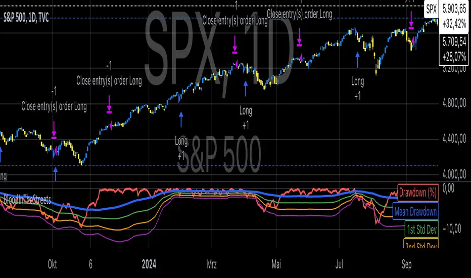
Bollinger Bands Mean Reversion by Kevin Davey Bollinger Bands Mean Reversion Strategy Description
The Bollinger Bands Mean Reversion Strategy is a popular trading approach based on the concept of volatility and market overreaction. The strategy leverages Bollinger Bands, which consist of an upper and lower band plotted around a central moving average, typically using standard deviations to measure volatility. When the price moves beyond these bands, it signals potential overbought or oversold conditions, and the strategy seeks to exploit a reversion back to the mean (the central band).
Strategy Components:
1. Bollinger Bands:
The bands are calculated using a 20-period Simple Moving Average (SMA) and a multiple (usually 2.0) of the standard deviation of the asset’s price over the same period. The upper band represents the SMA plus two standard deviations, while the lower band is the SMA minus two standard deviations. The distance between the bands increases with higher volatility and decreases with lower volatility.
2. Mean Reversion:
Mean reversion theory suggests that, over time, prices tend to move back toward their historical average. In this strategy, a buy signal is triggered when the price falls below the lower Bollinger Band, indicating a potential oversold condition. Conversely, the position is closed when the price rises back above the upper Bollinger Band, signaling an overbought condition.
Entry and Exit Logic:
Buy Condition: The strategy enters a long position when the price closes below the lower Bollinger Band, anticipating a mean reversion to the central band (SMA).
Sell Condition: The long position is exited when the price closes above the upper Bollinger Band, implying that the market is likely overbought and a reversal could occur.
This approach uses mean reversion principles, aiming to capitalize on short-term price extremes and volatility compression, often seen in sideways or non-trending markets. Scientific studies have shown that mean reversion strategies, particularly those based on volatility indicators like Bollinger Bands, can be effective in capturing small but frequent price reversals  .
Scientific Basis for Bollinger Bands:
Bollinger Bands, developed by John Bollinger, are widely regarded in both academic literature and practical trading as an essential tool for volatility analysis and mean reversion strategies. Research has shown that Bollinger Bands effectively identify relative price highs and lows, and can be used to forecast price volatility and detect potential breakouts . Studies in financial markets, such as those by Fernández-Rodríguez et al. (2003), highlight the efficacy of Bollinger Bands in detecting overbought or oversold conditions in various assets .
Who is Kevin Davey?
Kevin Davey is an award-winning algorithmic trader and highly regarded expert in developing and optimizing systematic trading strategies. With over 25 years of experience, Davey gained significant recognition after winning the prestigious World Cup Trading Championships multiple times, where he achieved triple-digit returns with minimal drawdown. His success has made him a key figure in algorithmic trading education, with a focus on disciplined and rule-based trading systems.

Chande Momentum Oscillator StrategyThe Chande Momentum Oscillator (CMO) Trading Strategy is based on the momentum oscillator developed by Tushar Chande in 1994. The CMO measures the momentum of a security by calculating the difference between the sum of recent gains and losses over a defined period. The indicator offers a means to identify overbought and oversold conditions, making it suitable for developing mean-reversion trading strategies (Chande, 1997).
Strategy Overview:
Calculation of the Chande Momentum Oscillator (CMO):
The CMO formula considers both positive and negative price changes over a defined period (commonly set to 9 days) and computes the net momentum as a percentage.
The formula is as follows:
CMO=100×(Sum of Gains−Sum of Losses)(Sum of Gains+Sum of Losses)
CMO=100×(Sum of Gains+Sum of Losses)(Sum of Gains−Sum of Losses)
This approach distinguishes the CMO from other oscillators like the RSI by using both price gains and losses in the numerator, providing a more symmetrical measurement of momentum (Chande, 1997).
Entry Condition:
The strategy opens a long position when the CMO value falls below -50, signaling an oversold condition where the price may revert to the mean. Research in mean-reversion, such as by Poterba and Summers (1988), supports this approach, highlighting that prices often revert after sharp movements due to overreaction in the markets.
Exit Conditions:
The strategy closes the long position when:
The CMO rises above 50, indicating that the price may have become overbought and may not provide further upside potential.
Alternatively, the position is closed 5 days after the buy signal is triggered, regardless of the CMO value, to ensure a timely exit even if the momentum signal does not reach the predefined level.
This exit strategy aligns with the concept of time-based exits, reducing the risk of prolonged exposure to adverse price movements (Fama, 1970).
Scientific Basis and Rationale:
Momentum and Mean-Reversion:
The strategy leverages the well-known phenomenon of mean-reversion in financial markets. According to research by Jegadeesh and Titman (1993), prices tend to revert to their mean over short periods following strong movements, creating opportunities for traders to profit from temporary deviations.
The CMO captures this mean-reversion behavior by monitoring extreme price conditions. When the CMO reaches oversold levels (below -50), it signals potential buying opportunities, whereas crossing overbought levels (above 50) indicates conditions for selling.
Market Efficiency and Overreaction:
The strategy takes advantage of behavioral inefficiencies and overreactions, which are often the drivers behind sharp price movements (Shiller, 2003). By identifying these extreme conditions with the CMO, the strategy aims to capitalize on the market’s tendency to correct itself when price deviations become too large.
Optimization and Parameter Selection:
The 9-day period used for the CMO calculation is a widely accepted timeframe that balances responsiveness and noise reduction, making it suitable for capturing short-term price fluctuations. Studies in technical analysis suggest that oscillators optimized over such periods are effective in detecting reversals (Murphy, 1999).
Performance and Backtesting:
The strategy's effectiveness is confirmed through backtesting, which shows that using the CMO as a mean-reversion tool yields profitable opportunities. The use of time-based exits alongside momentum-based signals enhances the reliability of the strategy by ensuring that trades are closed even when the momentum signal alone does not materialize.
Conclusion:
The Chande Momentum Oscillator Trading Strategy combines the principles of momentum measurement and mean-reversion to identify and capitalize on short-term price fluctuations. By using a widely tested oscillator like the CMO and integrating a systematic exit approach, the strategy effectively addresses both entry and exit conditions, providing a robust method for trading in diverse market environments.
References:
Chande, T. S. (1997). The New Technical Trader: Boost Your Profit by Plugging into the Latest Indicators. John Wiley & Sons.
Fama, E. F. (1970). Efficient Capital Markets: A Review of Theory and Empirical Work. The Journal of Finance, 25(2), 383-417.
Jegadeesh, N., & Titman, S. (1993). Returns to Buying Winners and Selling Losers: Implications for Stock Market Efficiency. The Journal of Finance, 48(1), 65-91.
Murphy, J. J. (1999). Technical Analysis of the Financial Markets: A Comprehensive Guide to Trading Methods and Applications. New York Institute of Finance.
Poterba, J. M., & Summers, L. H. (1988). Mean Reversion in Stock Prices: Evidence and Implications. Journal of Financial Economics, 22(1), 27-59.
Shiller, R. J. (2003). From Efficient Markets Theory to Behavioral Finance. Journal of Economic Perspectives, 17(1), 83-104.

Parent Session Sweeps + Alert Killzone Ranges with Parent Session Sweep
Key Features:
1. Multiple Session Support: The script tracks three major trading sessions - Asia, London, and New York. Users can customize the timing of these sessions.
2. Killzone Visualization: The strategy visually represents each session's range, either as filled boxes or lines, allowing traders to easily identify key price levels.
3. Parent Session Logic: The core of the strategy revolves around identifying a "parent" session - a session that encompasses the range of the following session. This parent session becomes the basis for potential trade setups.
4. Sweep and Reclaim Setups: The strategy looks for price movements that sweep (break above or below) the parent session's high or low, followed by a reclaim of that level. This price action often indicates a potential reversal.
5. Risk-Reward Filtering: Each potential setup is evaluated based on a user-defined minimum risk-reward ratio, ensuring that only high-quality trade opportunities are considered.
6. Candle Close Filter: An optional filter that checks the characteristics of the candle that reclaims the parent session level, adding an extra layer of confirmation to the setup.
7. Performance Tracking: The strategy keeps track of bullish and bearish setup success rates, providing valuable feedback on its performance over time.
8. Visual Aids: The script draws lines to mark the parent session's high and low, making it easy for traders to identify key levels.
How It Works:
1. The script continuously monitors price action across the defined sessions.
2. When a session fully contains the range of the next session, it's identified as a potential parent session.
3. The strategy then waits for price to sweep either the high or low of this parent session.
4. If a sweep occurs, it looks for a reclaim of the swept level within the parameters set by the user.
5. If a valid setup is identified, the script generates an alert and places a trade (if backtesting or running live).
6. The strategy continues to monitor the trade for either reaching the target (opposite level of the parent session) or hitting the stop loss.
Considerations for Signals:
- Sweep: A break of the parent session's high or low.
- Reclaim: A close back inside the parent session range after a sweep.
- Candle Characteristics: Optional filter for the reclaim candle (e.g., bullish candle for long setups).
- Risk-Reward: Each setup must meet or exceed the user-defined minimum risk-reward ratio.
- Session Timing: The strategy is sensitive to the defined session times, which should be set according to the trader's preferred time zone.
This strategy aims to capitalize on institutional order flow and liquidity patterns in the forex market, providing traders with a systematic approach to identifying potential reversal points with favorable risk-reward profiles.

Commitment of Trader %R StrategyThis Pine Script strategy utilizes the Commitment of Traders (COT) data to inform trading decisions based on the Williams %R indicator. The script operates in TradingView and includes various functionalities that allow users to customize their trading parameters.
Here’s a breakdown of its key components:
COT Data Import:
The script imports the COT library from TradingView to access historical COT data related to different trader groups (commercial hedgers, large traders, and small traders).
User Inputs:
COT data selection mode (e.g., Auto, Root, Base currency).
Whether to include futures, options, or both.
The trader group to analyze.
The lookback period for calculating the Williams %R.
Upper and lower thresholds for triggering trades.
An option to enable or disable a Simple Moving Average (SMA) filter.
Williams %R Calculation: The script calculates the Williams %R value, which is a momentum indicator that measures overbought or oversold levels based on the highest and lowest prices over a specified period.
SMA Filter: An optional SMA filter allows users to limit trades to conditions where the price is above or below the SMA, depending on the configuration.
Trade Logic: The strategy enters long positions when the Williams %R value exceeds the upper threshold and exits when the value falls below it. Conversely, it enters short positions when the Williams %R value is below the lower threshold and exits when the value rises above it.
Visual Elements: The script visually indicates the Williams %R values and thresholds on the chart, with the option to plot the SMA if enabled.
Commitment of Traders (COT) Data
The COT report is a weekly publication by the Commodity Futures Trading Commission (CFTC) that provides a breakdown of open interest positions held by different types of traders in the U.S. futures markets. It is widely used by traders and analysts to gauge market sentiment and potential price movements.
Data Collection: The COT data is collected from futures commission merchants and is published every Friday, reflecting positions as of the previous Tuesday. The report categorizes traders into three main groups:
Commercial Traders: These are typically hedgers (like producers and processors) who use futures to mitigate risk.
Non-Commercial Traders: Often referred to as speculators, these traders do not have a commercial interest in the underlying commodity but seek to profit from price changes.
Non-reportable Positions: Small traders who do not meet the reporting threshold set by the CFTC.
Interpretation:
Market Sentiment: By analyzing the positions of different trader groups, market participants can gauge sentiment. For instance, if commercial traders are heavily short, it may suggest they expect prices to decline.
Extreme Positions: Some traders look for extreme positions among non-commercial traders as potential reversal signals. For example, if speculators are overwhelmingly long, it might indicate an overbought condition.
Statistical Insights: COT data is often used in conjunction with technical analysis to inform trading decisions. Studies have shown that analyzing COT data can provide valuable insights into future price movements (Lund, 2018; Hurst et al., 2017).
Scientific References
Lund, J. (2018). Understanding the COT Report: An Analysis of Speculative Trading Strategies.
Journal of Derivatives and Hedge Funds, 24(1), 41-52. DOI:10.1057/s41260-018-00107-3
Hurst, B., O'Neill, R., & Roulston, M. (2017). The Impact of COT Reports on Futures Market Prices: An Empirical Analysis. Journal of Futures Markets, 37(8), 763-785.
DOI:10.1002/fut.21849
Commodity Futures Trading Commission (CFTC). (2024). Commitment of Traders. Retrieved from CFTC Official Website.

Bitcoin CME-Spot Z-Spread - Strategy [presentTrading]This time is a swing trading strategy! It measures the sentiment of the Bitcoin market through the spread of CME Bitcoin Futures and Bitfinex BTCUSD Spot prices. By applying Bollinger Bands to the spread, the strategy seeks to capture mean-reversion opportunities when prices deviate significantly from their historical norms
█ Introduction and How it is Different
The Bitcoin CME-Spot Bollinger Bands Strategy is designed to capture mean-reversion opportunities by exploiting the spread between CME Bitcoin Futures and Bitfinex BTCUSD Spot prices. The strategy uses Bollinger Bands to detect when the spread between these two correlated assets has deviated significantly from its historical norm, signaling potential overbought or oversold conditions.
What sets this strategy apart is its focus on spread trading between futures and spot markets rather than price-based indicators. By applying Bollinger Bands to the spread rather than individual prices, the strategy identifies price inefficiencies across markets, allowing traders to take advantage of the natural reversion to the mean that often occurs in these correlated assets.
BTCUSD 8hr Performance
█ Strategy, How It Works: Detailed Explanation
The strategy relies on Bollinger Bands to assess the volatility and relative deviation of the spread between CME Bitcoin Futures and Bitfinex BTCUSD Spot prices. Bollinger Bands consist of a moving average and two standard deviation bands, which help measure how much the spread deviates from its historical mean.
🔶 Spread Calculation:
The spread is calculated by subtracting the Bitfinex spot price from the CME Bitcoin futures price:
Spread = CME Price - Bitfinex Price
This spread represents the difference between the futures and spot markets, which may widen or narrow based on supply and demand dynamics in each market. By analyzing the spread, the strategy can detect when prices are too far apart (potentially overbought or oversold), indicating a trading opportunity.
🔶 Bollinger Bands Calculation:
The Bollinger Bands for the spread are calculated using a simple moving average (SMA) and the standard deviation of the spread over a defined period.
1. Moving Average (SMA):
The simple moving average of the spread (mu_S) over a specified period P is calculated as:
mu_S = (1/P) * sum(S_i from i=1 to P)
Where S_i represents the spread at time i, and P is the lookback period (default is 200 bars). The moving average provides a baseline for the normal spread behavior.
2. Standard Deviation:
The standard deviation (sigma_S) of the spread is calculated to measure the volatility of the spread:
sigma_S = sqrt((1/P) * sum((S_i - mu_S)^2 from i=1 to P))
3. Upper and Lower Bollinger Bands:
The upper and lower Bollinger Bands are derived by adding and subtracting a multiple of the standard deviation from the moving average. The number of standard deviations is determined by a user-defined parameter k (default is 2.618).
- Upper Band:
Upper Band = mu_S + (k * sigma_S)
- Lower Band:
Lower Band = mu_S - (k * sigma_S)
These bands provide a dynamic range within which the spread typically fluctuates. When the spread moves outside of these bands, it is considered overbought or oversold, potentially offering trading opportunities.
Local view
🔶 Entry Conditions:
- Long Entry: A long position is triggered when the spread crosses below the lower Bollinger Band, indicating that the spread has become oversold and is likely to revert upward.
Spread < Lower Band
- Short Entry: A short position is triggered when the spread crosses above the upper Bollinger Band, indicating that the spread has become overbought and is likely to revert downward.
Spread > Upper Band
🔶 Risk Management and Profit-Taking:
The strategy incorporates multi-step take profits to lock in gains as the trade moves in favor. The position is gradually reduced at predefined profit levels, reducing risk while allowing part of the trade to continue running if the price keeps moving favorably.
Additionally, the strategy uses a hold period exit mechanism. If the trade does not hit any of the take-profit levels within a certain number of bars, the position is closed automatically to avoid excessive exposure to market risks.
█ Trade Direction
The trade direction is based on deviations of the spread from its historical norm:
- Long Trade: The strategy enters a long position when the spread crosses below the lower Bollinger Band, signaling an oversold condition where the spread is expected to narrow.
- Short Trade: The strategy enters a short position when the spread crosses above the upper Bollinger Band, signaling an overbought condition where the spread is expected to widen.
These entries rely on the assumption of mean reversion, where extreme deviations from the average spread are likely to revert over time.
█ Usage
The Bitcoin CME-Spot Bollinger Bands Strategy is ideal for traders looking to capitalize on price inefficiencies between Bitcoin futures and spot markets. It’s especially useful in volatile markets where large deviations between futures and spot prices occur.
- Market Conditions: This strategy is most effective in correlated markets, like CME futures and spot Bitcoin. Traders can adjust the Bollinger Bands period and standard deviation multiplier to suit different volatility regimes.
- Backtesting: Before deployment, backtesting the strategy across different market conditions and timeframes is recommended to ensure robustness. Adjust the take-profit steps and hold periods to reflect the trader’s risk tolerance and market behavior.
█ Default Settings
The default settings provide a balanced approach to spread trading using Bollinger Bands but can be adjusted depending on market conditions or personal trading preferences.
🔶 Bollinger Bands Period (200 bars):
This defines the number of bars used to calculate the moving average and standard deviation for the Bollinger Bands. A longer period smooths out short-term fluctuations and focuses on larger, more significant trends. Adjusting the period affects the responsiveness of the strategy:
- Shorter periods (e.g., 100 bars): Makes the strategy more reactive to short-term market fluctuations, potentially generating more signals but increasing the risk of false positives.
- Longer periods (e.g., 300 bars): Focuses on longer-term trends, reducing the frequency of trades and focusing only on significant deviations.
🔶 Standard Deviation Multiplier (2.618):
The multiplier controls how wide the Bollinger Bands are around the moving average. By default, the bands are set at 2.618 standard deviations away from the average, ensuring that only significant deviations trigger trades.
- Higher multipliers (e.g., 3.0): Require a more extreme deviation to trigger trades, reducing trade frequency but potentially increasing the accuracy of signals.
- Lower multipliers (e.g., 2.0): Make the bands narrower, increasing the number of trade signals but potentially decreasing their reliability.
🔶 Take-Profit Levels:
The strategy has four take-profit levels to gradually lock in profits:
- Level 1 (3%): 25% of the position is closed at a 3% profit.
- Level 2 (8%): 20% of the position is closed at an 8% profit.
- Level 3 (14%): 15% of the position is closed at a 14% profit.
- Level 4 (21%): 10% of the position is closed at a 21% profit.
Adjusting these take-profit levels affects how quickly profits are realized:
- Lower take-profit levels: Capture gains more quickly, reducing risk but potentially cutting off larger profits.
- Higher take-profit levels: Let trades run longer, aiming for bigger gains but increasing the risk of price reversals before profits are locked in.
🔶 Hold Days (20 bars):
The strategy automatically closes the position after 20 bars if none of the take-profit levels are hit. This feature prevents trades from being held indefinitely, especially if market conditions are stagnant. Adjusting this:
- Shorter hold periods: Reduce the duration of exposure, minimizing risks from market changes but potentially closing trades too early.
- Longer hold periods: Allow trades to stay open longer, increasing the chance for mean reversion but also increasing exposure to unfavorable market conditions.
By understanding how these default settings affect the strategy’s performance, traders can optimize the Bitcoin CME-Spot Bollinger Bands Strategy to their preferences, adapting it to different market environments and risk tolerances.