Multifractal Forecast [ScorsoneEnterprises]

Multifractal Forecast [ScorsoneEnterprises] Indicator

The Multifractal Forecast is an indicator designed to model and forecast asset price movements using a multifractal framework. It uses concepts from fractal geometry and stochastic processes, specifically the Multifractal Model of Asset Returns (MMAR) and fractional Brownian motion (fBm), to generate price forecasts based on historical price data. The indicator visualizes potential future price paths as colored lines, providing traders with a probabilistic view of price trends over a specified trading time scale. Below is a detailed breakdown of the indicator’s functionality, inputs, calculations, and visualization.

Overview
Purpose: The indicator forecasts future price movements by simulating multiple price paths based on a multifractal model, which accounts for the complex, non-linear behavior of financial markets.

Key Concepts:
Multifractal Model of Asset Returns (MMAR): Models price movements as a multifractal process, capturing varying degrees of volatility and self-similarity across different time scales.

Fractional Brownian Motion (fBm): A generalization of Brownian motion that incorporates long-range dependence and self-similarity, controlled by the Hurst exponent.

Binomial Cascade: Used to model trading time, introducing heterogeneity in time scales to reflect market activity bursts.

Hurst Exponent: Measures the degree of long-term memory in the price series (persistence, randomness, or mean-reversion).

Rescaled Range (R/S) Analysis: Estimates the Hurst exponent to quantify the fractal nature of the price series.

Inputs
The indicator allows users to customize its behavior through several input parameters, each influencing the multifractal model and forecast generation:
Maximum Lag (max_lag):
Type: Integer

Default: 50

Minimum: 5

Purpose: Determines the maximum lag used in the rescaled range (R/S) analysis to calculate the Hurst exponent. A higher lag increases the sample size for Hurst estimation but may smooth out short-term dynamics.

2 to the n values in the Multifractal Model (n):
Type: Integer

Default: 4

Purpose: Defines the resolution of the multifractal model by setting the size of arrays used in calculations (N = 2^n). For example, n=4 results in N=16 data points. Larger n increases computational complexity and detail but may exceed Pine Script’s array size limits (capped at 100,000).

Multiplier for Binomial Cascade (m):
Type: Float

Default: 0.8

Purpose: Controls the asymmetry in the binomial cascade, which models trading time. The multiplier m (and its complement 2.0 - m) determines how mass is distributed across time scales. Values closer to 1 create more balanced cascades, while values further from 1 introduce more variability.

Length Scale for fBm (L):
Type: Float

Default: 100,000.0

Purpose: Scales the fractional Brownian motion output, affecting the amplitude of simulated price paths. Larger values increase the magnitude of forecasted price movements.

Cumulative Sum (cum):
Type: Integer (0 or 1)

Default: 1

Purpose: Toggles whether the fBm output is cumulatively summed (1=On, 0=Off). When enabled, the fBm series is accumulated to simulate a price path with memory, resembling a random walk with long-range dependence.

Trading Time Scale (T):
Type: Integer

Default: 5

Purpose: Defines the forecast horizon in bars (20 bars into the future). It also scales the binomial cascade’s output to align with the desired trading time frame.

Number of Simulations (num_simulations):
Type: Integer

Default: 5

Minimum: 1

Purpose: Specifies how many forecast paths are simulated and plotted. More simulations provide a broader range of possible price outcomes but increase computational load.

Core Calculations
The indicator combines several mathematical and statistical techniques to generate price forecasts. Below is a step-by-step explanation of its calculations:
Log Returns (lgr):
The indicator calculates log returns as math.log(close / close[1]) when both the current and previous close prices are positive. This measures the relative price change in a logarithmic scale, which is standard for financial time series analysis to stabilize variance.

Hurst Exponent Estimation (get_hurst_exponent):
Purpose: Estimates the Hurst exponent (H) to quantify the degree of long-term memory in the price series.

Method: Uses rescaled range (R/S) analysis:
For each lag from 2 to max_lag, the function calc_rescaled_range computes the rescaled range:
Calculate the mean of the log returns over the lag period.

Compute the cumulative deviation from the mean.

Find the range (max - min) of the cumulative deviation.

Divide the range by the standard deviation of the log returns to get the rescaled range.

The log of the rescaled range (log(R/S)) is regressed against the log of the lag (log(lag)) using the polyfit_slope function.

The slope of this regression is the Hurst exponent (H).

Interpretation:
H = 0.5: Random walk (no memory, like standard Brownian motion).

H > 0.5: Persistent behavior (trends tend to continue).

H < 0.5: Mean-reverting behavior (price tends to revert to the mean).

Fractional Brownian Motion (get_fbm):
Purpose: Generates a fractional Brownian motion series to model price movements with long-range dependence.

Inputs: n (array size 2^n), H (Hurst exponent), L (length scale), cum (cumulative sum toggle).

Method:
Computes covariance for fBm using the formula: 0.5 * (|i+1|^(2H) - 2 * |i|^(2H) + |i-1|^(2H)).

Uses Hosking’s method (referenced from Columbia University’s implementation) to generate fBm:
Initializes arrays for covariance (cov), intermediate calculations (phi, psi), and output.

Iteratively computes the fBm series by incorporating a random term scaled by the variance (v) and covariance structure.

Applies scaling based on L / N^H to adjust the amplitude.

Optionally applies cumulative summation if cum = 1 to produce a path with memory.

Output: An array of 2^n values representing the fBm series.

Binomial Cascade (get_binomial_cascade):
Purpose: Models trading time (theta) to account for non-uniform market activity (e.g., bursts of volatility).

Inputs: n (array size 2^n), m (multiplier), T (trading time scale).

Method:
Initializes an array of size 2^n with values of 1.0.

Iteratively applies a binomial cascade:
For each block (from 0 to n-1), splits the array into segments.

Randomly assigns a multiplier (m or 2.0 - m) to each segment, redistributing mass.

Normalizes the array by dividing by its sum and scales by T.

Checks for array size limits to prevent Pine Script errors.

Output: An array (theta) representing the trading time, which warps the fBm to reflect market activity.

Interpolation (interpolate_fbm):
Purpose: Maps the fBm series to the trading time scale to produce a forecast.

Method:
Computes the cumulative sum of theta and normalizes it to [0, 1].

Interpolates the fBm series linearly based on the normalized trading time.

Ensures the output aligns with the trading time scale (T).

Output: An array of interpolated fBm values representing log returns over the forecast horizon.

Price Path Generation:
For each simulation (up to num_simulations):
Generates an fBm series using get_fbm.

Interpolates it with the trading time (theta) using interpolate_fbm.

Converts log returns to price levels:
Starts with the current close price.

For each step i in the forecast horizon (T), computes the price as prev_price * exp(log_return).

Output: An array of price levels for each simulation.

Visualization:
Trigger: Updates every T bars when the bar state is confirmed (barstate.isconfirmed).

Process:
Clears previous lines from line_array.

For each simulation, plots a line from the current bar’s close price to the forecasted price at bar_index + T.

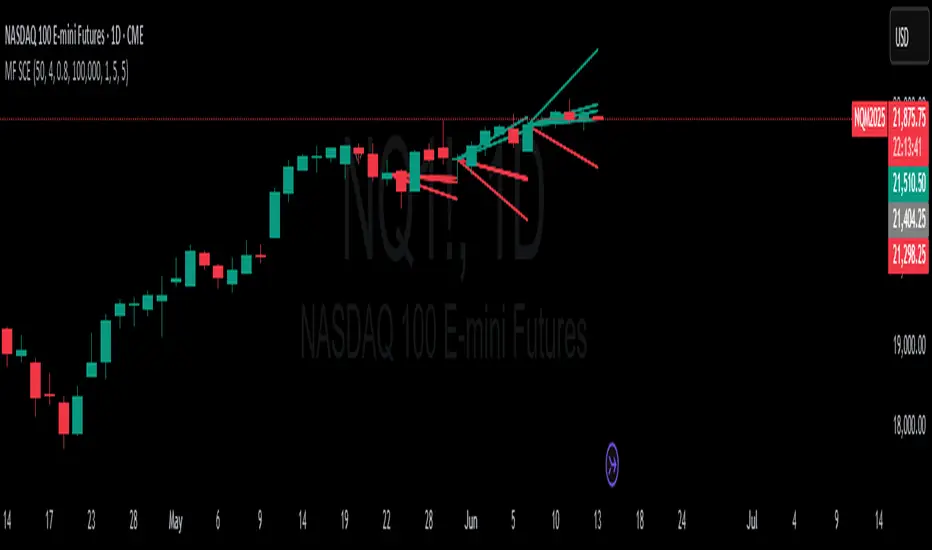
Colors the line using a gradient (color.from_gradient) based on the final forecasted price relative to the minimum and maximum forecasted prices across all simulations (red for lower prices, teal for higher prices).

Output: Multiple colored lines on the chart, each representing a possible price path over the next T bars.

How It Works on the Chart
Initialization: On each bar, the indicator calculates the Hurst exponent (H) using historical log returns and prepares the trading time (theta) using the binomial cascade.

Forecast Generation: Every T bars, it generates num_simulations price paths:
Each path starts at the current close price.

Uses fBm to model log returns, warped by the trading time.

Converts log returns to price levels.

Plotting: Draws lines from the current bar to the forecasted price T bars ahead, with colors indicating relative price levels.

Dynamic Updates: The forecast updates every T bars, replacing old lines with new ones based on the latest price data and calculations.

Key Features
Multifractal Modeling: Captures complex market dynamics by combining fBm (long-range dependence) with a binomial cascade (non-uniform time).

Customizable Parameters: Allows users to adjust the forecast horizon, model resolution, scaling, and number of simulations.

Probabilistic Forecast: Multiple simulations provide a range of possible price outcomes, helping traders assess uncertainty.

Visual Clarity: Gradient-colored lines make it easy to distinguish bullish (teal) and bearish (red) forecasts.

Potential Use Cases
Trend Analysis: Identify potential price trends or reversals based on the direction and spread of forecast lines.

Risk Assessment: Evaluate the range of possible price outcomes to gauge market uncertainty.

Volatility Analysis: The Hurst exponent and binomial cascade provide insights into market persistence and volatility clustering.

Limitations
Computational Intensity: Large values of n or num_simulations may slow down execution or hit Pine Script’s array size limits.

Randomness: The binomial cascade and fBm rely on random terms (math.random), which may lead to variability between runs.

Assumptions: The model assumes log-normal price movements and fractal behavior, which may not always hold in extreme market conditions.

Adjusting Inputs:
Set max_lag based on the desired depth of historical analysis.

Adjust n for model resolution (start with 4–6 to avoid performance issues).

Tune m to control trading time variability (0.5–1.5 is typical).

Set L to scale the forecast amplitude (experiment with values like 10,000–1,000,000).

Choose T based on your trading horizon (20 for short-term, 50 for longer-term for example).

Select num_simulations for the number of forecast paths (5–10 is reasonable for visualization).

Interpret Output:
Teal lines suggest bullish scenarios, red lines suggest bearish scenarios.

A wide spread of lines indicates high uncertainty; convergence suggests a stronger trend.

Monitor Updates: Forecasts update every T bars, so check the chart periodically for new projections.

Chart Examples


This is a daily SPY chart with default settings. We see the simulations being done every T bars and they provide a range for us to analyze with a few simulations still in the range.


On this intraday COCOA chart I modified the Length Scale for fBm, L, parameter to be 1000 from 100000. Adjusting the parameter as you switch between timeframes can give you more contextual simulations.


On ETHUSD I modified the L to be 1000000 to have a more contextual set of simulations with crypto's volatile nature.


With L at 100000 we see the range for TLT is correctly simulated. The recent pop stays within the bounds of the highest simulation. Note this is a cherry picked example to show the power and potential of these simulations.

Technical Notes
Error Handling: The script includes checks for array size limits and division by zero (math.abs(denominator) > 1e-10, v := math.max(v, 1e-10)).

External Reference: The fBm implementation is based on Hosking’s method (columbia.edu/~ad3217/fbm/hosking.c), ensuring a robust algorithm.

Conclusion
The Multifractal Forecast [ScorsoneEnterprises] is a powerful tool for traders seeking to model complex market dynamics using a multifractal framework. By combining fBm, binomial cascades, and Hurst exponent analysis, it generates probabilistic price forecasts that account for long-range dependence and non-uniform market activity. Its customizable inputs and clear visualizations make it suitable for both technical analysis and strategy development, though users should be mindful of its computational demands and parameter sensitivity. For optimal use, experiment with input settings and validate forecasts against other technical indicators or market conditions.