Straddle / strangle buy or sell indicatorStraddle / strangle buy or sell indicator developed by Chobotaru Brothers.
You need to have basic knowledge in option trading to use this indicator!
The indicator shows P&L lines of the options strategy. Use only for stocks since the mathematical model of options for Future instruments is different from stocks. Plus, the days' representation in futures is also different from stocks (stocks have fewer days than futures ).
***Each strategy in options is based on different mathematical equations, use this indicator only for the strategy in the headline.***
What does the indicator do?
The indicator is based on the Black-Scholes model, which uses partial differential equations to determine the option pricing. Due to options non-linear behavior, it is hard to visualize the option price. The indicator calculates the solutions of the Black-Scholes equation and plots them on the chart so traders can view how the option pricing will behave.
How the indicator does it?
The indicator uses five values (four dominants and one less dominant) to solve the Black-Scholes equation. The values are stock price, the strike price of the option, time to expiration, risk-free interest rate, and implied volatility .
How the indicator help the users?
-View the risks and rewards so you can know the profit targets in advance which means you can compare different options in different strikes.
-View the volatility change impact so you can know the risk and the P&L changes in case of a change in the volatility over the life of the option before you enter the trade.
-View the passage of time impact so you can know where and when you could realize a profit.
-Multi-timeframes so you can stay on the same chart (Daily and below).
All these features are to help the user improve his analysis while trading options.
How to use it?
The user needs to obtain from the “option chain” the following inputs:
-Buy or sell (the strategy)
- Straddle/strangle price bought/sold: enter the price that you bought/sold one options strategy.
-Instrument price when bought/sold: the stock price when you bought/sold the options strategy.
-Upper strike price: the upper strike price of the options strategy.
-Lower strike price: the lower strike price of the options strategy.
-Interest rate: find the risk-free interest rate from the U.S. DEPARTMENT OF THE TREASURY. Example: for 2% interest rate, input: 0.02.
-Days to expire: how many days until the option expires.
-Volatility: the implied volatility of the option bought/sold. Example: for 45% implied volatility , input: 0.45.
-Day of entry: A calendar day of the month that the option bought/sold.
-Month of entry: Calendar month the option bought/sold.
-Year of entry: Calendar year the option bought/sold.
-Risk to reward: Profit/loss line defined by the user. Minimum input (-0.95) ; maximum input (3).
Example: If the strategy was bought, -0.95 means, 95% of the options strategy value is lost (unrealized). If the strategy was bought, 3 means, the risk to reward is 3.
After entering all the inputs, press Ok and you should see “Calculation Complete” on the chart.
The user should not change the entry date and days to expire inputs as time passes after he entered the trade.
How to access the indicator?
Use the link below to obtain access to the indicator
在腳本中搜尋"implied"

Call Bear Spread indicatorCall bear spread indicator developed by Chobotaru Brothers.
You need to have basic knowledge in option trading to use this indicator!
This spread is a CREDIT SPREAD.
The indicator shows P&L lines of the options strategy. Use only for stocks since the mathematical model of options for Future instruments is different from stocks. Plus, the days' representation in futures is also different from stocks (stocks have fewer days than futures ).
***Each strategy in options is based on different mathematical equations, use this indicator only for the strategy in the headline.***
What does the indicator do?
The indicator is based on the Black-Scholes model, which uses partial differential equations to determine the option pricing. Due to options non-linear behavior, it is hard to visualize the option price. The indicator calculates the solutions of the Black-Scholes equation and plots them on the chart so traders can view how the option pricing will behave.
How the indicator does it?
The indicator uses five values (four dominants and one less dominant) to solve the Black-Scholes equation. The values are stock price, the strike price of the option, time to expiration, risk-free interest rate, and implied volatility .
How the indicator help the users?
-View the risks and rewards so you can know the profit targets in advance which means you can compare different options in different strikes.
-View the volatility change impact so you can know the risk and the P&L changes in case of a change in the volatility over the life of the option before you enter the trade.
-View the passage of time impact so you can know where and when you could realize a profit.
-Multi-timeframes so you can stay on the same chart (Daily and below).
All these features are to help the user improve his analysis while trading options.
How to use it?
The user needs to obtain from the “option chain” the following inputs:
- Call spread price (Credit): The credit received for one unit of options strategy.
-Instrument price when entered spread: the stock price when you enter the options strategy.
-Upper strike price: the upper strike price of the options strategy.
-Lower strike price: the lower strike price of the options strategy.
-Interest rate: find the risk-free interest rate from the U.S. DEPARTMENT OF THE TREASURY. Example: for 2% interest rate, input: 0.02.
-Days to expire: how many days until the option expires.
-Volatility: the implied volatility of the option bought/sold. Example: for 45% implied volatility , input: 0.45.
-Day of entry: A calendar day of the month that the option bought/sold.
-Month of entry: Calendar month the option bought/sold.
-Year of entry: Calendar year the option bought/sold.
-% of Max Profit/Loss: Profit/loss line defined by the user. Minimum input (-0.95) ; maximum input (0.95).
Example: In this spread, -0.95 means, 95% of the options strategy maximum loss is reached and, 0.95 means, 95% of the options strategy maximum profit is reached.
After entering all the inputs, press Ok and you should see “Calculation Complete” on the chart.
The user should not change the entry date and days to expire inputs as time passes after he entered the trade.
How to access the indicator?
Use the link below to obtain access to the indicator

Call bull spread indicatorCall bull spread indicator developed by Chobotaru Brothers.
You need to have basic knowledge in option trading to use this indicator!
This spread is a DEBIT SPREAD.
The indicator shows P&L lines of the options strategy. Use only for stocks since the mathematical model of options for Future instruments is different from stocks. Plus, the days' representation in futures is also different from stocks (stocks have fewer days than futures ).
***Each strategy in options is based on different mathematical equations, use this indicator only for the strategy in the headline.***
What does the indicator do?
The indicator is based on the Black-Scholes model, which uses partial differential equations to determine the option pricing. Due to options non-linear behavior, it is hard to visualize the option price. The indicator calculates the solutions of the Black-Scholes equation and plots them on the chart so traders can view how the option pricing will behave.
How the indicator does it?
The indicator uses five values (four dominants and one less dominant) to solve the Black-Scholes equation. The values are stock price, the strike price of the option, time to expiration, risk-free interest rate, and implied volatility .
How the indicator help the users?
-View the risks and rewards so you can know the profit targets in advance which means you can compare different options in different strikes.
-View the volatility change impact so you can know the risk and the P&L changes in case of a change in the volatility over the life of the option before you enter the trade.
-View the passage of time impact so you can know where and when you could realize a profit.
-Multi-timeframes so you can stay on the same chart (Daily and below).
All these features are to help the user improve his analysis while trading options.
How to use it?
The user needs to obtain from the “option chain” the following inputs:
- Call spread price (Debit): The debit paid for one unit of options strategy.
-Instrument price when entered spread: the stock price when you enter the options strategy.
-Upper strike price: the upper strike price of the options strategy.
-Lower strike price: the lower strike price of the options strategy.
-Interest rate: find the risk-free interest rate from the U.S. DEPARTMENT OF THE TREASURY. Example: for 2% interest rate, input: 0.02.
-Days to expire: how many days until the option expires.
-Volatility: the implied volatility of the option bought/sold. Example: for 45% implied volatility , input: 0.45.
-Day of entry: A calendar day of the month that the option bought/sold.
-Month of entry: Calendar month the option bought/sold.
-Year of entry: Calendar year the option bought/sold.
-% of Max Profit/Loss: Profit/loss line defined by the user. Minimum input (-0.95) ; maximum input (0.95).
Example: In this spread, -0.95 means, 95% of the options strategy maximum loss is reached and, 0.95 means, 95% of the options strategy maximum profit is reached.
After entering all the inputs, press Ok and you should see “Calculation Complete” on the chart.
The user should not change the entry date and days to expire inputs as time passes after he entered the trade.
How to access the indicator?
Use the link below to obtain access to the indicator

Put option buy or sell indicatorPut option indicator developed by Chobotaru Brothers.
You need to have basic knowledge in option trading to use this indicator!
The indicator shows P&L lines of the options strategy. Use only for stocks since the mathematical model of options for Future instruments is different from stocks. Plus, the days' representation in futures is also different from stocks (stocks have fewer days than futures ).
***Each strategy in options is based on different mathematical equations, use this indicator only for the strategy in the headline.***
What does the indicator do?
The indicator is based on the Black-Scholes model, which uses partial differential equations to determine the option pricing. Due to options non-linear behavior, it is hard to visualize the option price. The indicator calculates the solutions of the Black-Scholes equation and plots them on the chart so traders can view how the option pricing will behave.
How the indicator does it?
The indicator uses five values (four dominants and one less dominant) to solve the Black-Scholes equation. The values are stock price, the strike price of the option, time to expiration, risk-free interest rate, and implied volatility .
How the indicator help the users?
-View the risks and rewards so you can know the profit targets in advance which means you can compare different options in different strikes.
-View the volatility change impact so you can know the risk and the P&L changes in case of a change in the volatility over the life of the option before you enter the trade.
-View the passage of time impact so you can know where and when you could realize a profit.
-Multi-timeframes so you can stay on the same chart (Daily and below).
All these features are to help the user improve his analysis while trading options.
How to use it?
The user needs to obtain from the “option chain” the following inputs:
-Buy or sell (the strategy)
-The option price bought: at what price did you bought/sold one option.
-Instrument price when bought: the stock price when you bought/sold the option.
-Strike price: the strike price of the option.
-Interest rate: find the risk-free interest rate from the U.S. DEPARTMENT OF THE TREASURY. Example: for 2% interest rate, input: 0.02.
-Days to expire: how many days until the option expires.
-Volatility: the implied volatility of the option bought/sold. Example: for 45% implied volatility , input: 0.45.
-Day of entry: A calendar day of the month that the option bought/sold.
-Month of entry: Calendar month the option bought/sold.
-Year of entry: Calendar year the option bought/sold.
-Risk to reward: Profit/loss line defined by the user. Minimum input (-0.95) ; maximum input (3).
Example: If an option was bought, -0.95 means, 95% of the option value is lost (unrealized). If an option was bought, 3 means, the risk to reward is 3.
After entering all the inputs, press Ok and you should see “Calculation Complete” on the chart.
The user should not change the entry date and days to expire inputs as time passes after he entered the trade.
How to access the indicator?
Use the link below to obtain access to the indicator
Call option buy or sell indicatorCall option indicator developed by Chobotaru Brothers.
You need to have basic knowledge in option trading to use this indicator!
The indicator shows P&L lines of the options strategy. Use only for stocks since the mathematical model of options for Future instruments is different from stocks. Plus, the days' representation in futures is also different from stocks (stocks have fewer days than futures ).
***Each strategy in options is based on different mathematical equations, use this indicator only for the strategy in the headline.***
What does the indicator do?
The indicator is based on the Black-Scholes model, which uses partial differential equations to determine the option pricing. Due to options non-linear behavior, it is hard to visualize the option price. The indicator calculates the solutions of the Black-Scholes equation and plots them on the chart so traders can view how the option pricing will behave.
How the indicator does it?
The indicator uses five values (four dominants and one less dominant) to solve the Black-Scholes equation. The values are stock price, the strike price of the option, time to expiration, risk-free interest rate, and implied volatility .
How the indicator help the users?
-View the risks and rewards so you can know the profit targets in advance which means you can compare different options in different strikes.
-View the volatility change impact so you can know the risk and the P&L changes in case of a change in the volatility over the life of the option before you enter the trade.
-View the passage of time impact so you can know where and when you could realize a profit.
-Multi-timeframes so you can stay on the same chart (Daily and below).
All these features are to help the user improve his analysis while trading options.
How to use it?
The user needs to obtain from the “option chain” the following inputs:
-Buy or sell (the strategy)
-The option price bought: at what price did you bought/sold one option.
-Instrument price when bought: the stock price when you bought/sold the option.
-Strike price: the strike price of the option.
-Interest rate: find the risk-free interest rate from the U.S. DEPARTMENT OF THE TREASURY. Example: for 2% interest rate, input: 0.02.
-Days to expire: how many days until the option expires.
-Volatility: the implied volatility of the option bought/sold. Example: for 45% implied volatility , input: 0.45.
-Day of entry: A calendar day of the month that the option bought/sold.
-Month of entry: Calendar month the option bought/sold.
-Year of entry: Calendar year the option bought/sold.
-Risk to reward: Profit/loss line defined by the user. Minimum input (-0.95) ; maximum input (3).
Example: If an option was bought, -0.95 means, 95% of the option value is lost (unrealized). If an option was bought, 3 means, the risk to reward is 3.
After entering all the inputs, press Ok and you should see “Calculation Complete” on the chart.
The user should not change the entry date and days to expire inputs as time passes after he entered the trade.
How to access the indicator?
Use the link below to obtain access to the indicator
Synthetic VX3! & VX4! continuous /VX futuresTradingView is missing continuous 3rd and 4th month VIX (/VX) futures, so I decided to try to make a synthetic one that emulates what continuous maturity futures would look like. This is useful for backtesting/historical purposes as it enables traders to see how their further out VX contracts would've performed vs the front month contract.
The indicator pulls actual realtime data (if you subscribe to the CBOE data package) or 15 minute delayed data for the VIX spot (the actual non-tradeable VIX index), the continuous front month (VX1!), and the continuous second month (VX2!) continually rolled contracts. Then the indicator's script applies a formula to fairly closely estimate how 3rd and 4th month continuous contracts would've moved.
It uses an exponential mean‑reversion to a long‑run level formula using:
σ(T) = θ+(σ0−θ)e−kT
You can expect it to be off by ~5% or so (in times of backwardation it might be less accurate).

MeanReversion - LogReturn/Vola ZScoreShows the z-Score of log-return (blue line) and volatility (black line). In statistics, the z-score is the number of standard deviations by which a value of a raw score is above or below the mean value.
This indicator aggregates z-score based on two indicators:
MeanReversion by Logarithmic Returns
MeanReversion by Volatility
Change the time period in bars for longer or shorter time frames. At a daily chart 252 mean on trading year, 21 mean one trading month.

Rectified BB% for option tradingThis indicator shows the bollinger bands against the price all expressed in percentage of the mean BB value. With one sight you can see the amplitude of BB and the variation of the price, evaluate a reenter of the price in the BB.
The relative price is visualized as a candle with open/high/low/close value exspressed as percentage deviation from the BB mean
The indicator include a modified RSI, remapped from 0/100 to -100/100.
You can choose the BB parameters (length, standard deviation multiplier) and the RSI parameter (length, overbougth threshold, ovrsold threshold)
You can exclude/include the candles and the RSI line.
The indicator can be used to sell options when the volatility is high (the bollinger band is wide) and the price is reentering inside the bands.
If the price is forming a supply or demand area it can be a good opportunity to sell a bull put or a bear call
The RSI can be used as confirm of the supply/demand formation
If the bollinger band is narrow and the RSI is overbought/oversold it indicate a better opportunity to buy options
the indicator is designed to work with daily timeframe and default parameters.

ATR and IV Volatility TableThis is a volatility tool designed to get the daily bottom and top values calculated using a daily ATR and IV values.
ATR values can be calculated directly, however for IV I recommend to take the values from external sources for the asset that you want to trade.
Regarding of the usage, I always recommend to go at the end of the previous close day of the candle(with replay function) or beginning of the daily open candle and get the expected values for movements.
For example for 26April for SPX, we have an ATR of 77 points and the close of the candle was 4296.
So based on ATR for 27 April our TOP is going to be 4296 + 77 , while our BOT is going to be 4296-77
At the same time lets assume the IV for today is going to be around 25% -> this is translated to 25 / (sqrt (252)) = 1.57 aprox
So based on IV our TOP is going to be 4296 + 4296 * 0.0157 , while our BOT is going to be 4296 - 4296 * 0.0157
I found out from my calculations that 80-85% of the times these bot and top points act as an amazing support and resistence points for day trading, so I fully recommend you to start including them into your analysis.
If you have any questions let me know !
vx_termsUSAGE
--------
This script helps train your intuition for changes in the VX term structure. I recommend using it on the VIX chart, so you can compare changes in the terms to changes in VIX. It's also nice for calendar spread traders who want to get a feel for the same changes.
1. Select a day, month, and year using the inputs
2. Observe the data table.
3. Open the input again and increment or decrement the day (and month, year as necessary).
4. Click "Ok".
5. Click to deselect the indicator, which allows the chart to load new data.
6. The data table will be reloaded with the next/previous day's data.
The data table has the following columns:
- contract: the VX contracts, in sequence. refer to the CBOE for month codes (F for January, etc.)
- close: the closing price of the contract.
- ma:mb: the spread (difference) between this row and the next row.
- ma:mb chg: the spread's change from prior close.
For example, given the following values for the first two columns:
VXQ2021, 16.5, -3.1, -0.2
VXU2021, 19.6, ..., ...
The front month (Q = august) closed at 16.5, $3.1 below the s\September contract. The negative spread enlarged by $0.20 from $2.90 on the previous trading day.
BUGS, ODDITIES, AND LIMITATIONS:
-------------------------------------------
- The first column will be greyed out after expiration day, which is the 3rd Tuesday of that month. Unfortunately, I can't load the next month's contract due to some limitations with TV.
- The active date is highlighted with a yellow background. When a non-trading date is selected, the highlight will disappear. However, the data table will sometimes fill with the nearest trading date, prematurely. No worries, just know that the data is probably for the previous Friday.
- The script is clunky and slow, but this is the best I can do with TV. Hopefully they add more continuous contracts or allow true dynamic symbol loading.
SPECIAL THANKS:
---------------------
Thanks to HeWhoMustNotBeNamed for helping me get through some messiness. Very helpful guy.
www.tradingview.com

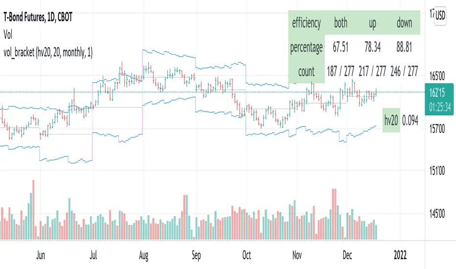
vol_bracketThis simple script shows an "N" standard deviation volatility bracket, anchored at the opening price of the current month, week, or quarter. This anchor is meant to coincide roughly with the expiration of options issued at the same interval. You can choose between a manually-entered IV or the hv30 volatility model.
Unlike my previous scripts, which all show the volatility bracket as a rolling figure, the anchor helps to visualize the volatility estimate in relation to price as it ranges over the (approximate) lifetime of a single, real contract.
VIX Term StructureThis script allows users to visualize the state of the VIX Futures Term Structure. The user is able to select from five CBOE VIX Indices; VIX, VIX9D, VIX3M, VIX6M, and VIX1Y and the script will color the candles based on the price relationship between selected indices. Visit the CBOE website for more info on how the various VIX indices are calculated.

Volatility Price TargetsPrints lines on the chart marking the price points for the standard deviation move using historical volatility. This script was born out of a need to easily spot target points for the wings of my Iron Condor Options trades. The study only shows on the Daily chart. Volatility is calculated based on the standard deviation of the daily returns of price. Price targets are calculated off yesterday's closing price and will not reprint.
Inputs
Days to Expiration - allow you to enter the number of days to expiration for the option, default is 30 for those monthly options traders but can be adjusted to your desire.
Standard Deviation - you can enter the number of deviations for which to calculate the price points 1,2, or 3.
Days in Year - you can adjust the number of days in the year used to calculate the daily volatility multiplier.


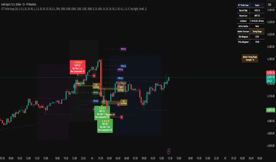
ICT Turtle SoupICT Turtle Soup identifies classic “failed breakout” reversals after liquidity sweeps of recent highs/lows, then augments the setup with volume validation, market structure context, Kill Zone (session) filters, Order Blocks (OB), Fair Value Gaps (FVG), OTE (61.8–78.6%) zones, and optional risk targets (SL/TP 1:1, 1:2, 1:3). A compact dashboard summarizes current context (recent high/low, lookbacks, active session, structure state, mitigation counts).
What the Script Does
⦁ Detects Turtle Soup events: Price breaks a prior swing extreme and then quickly reverses back inside the range.
⦁ Grades signal quality: Factors include reversal speed, volume confirmation, breakout magnitude, and consecutive patterns.
⦁ Overlays market context: Trend/range classification (ADX / MA / ATR Bands / Combined), Kill Zones (Asian/London/NY), and time-of-day filters.
⦁ Marks IMB / mitigation zones: Draws Order Blocks and Fair Value Gaps, with optional live mitigation tracking and fading/removal on mitigation.
⦁ Shows OTE zones (61.8–78.6%) after confirmed reversals to highlight potential pullback entries.
⦁ Plots risk management guides: Optional SL buffer below/above reversal wick and TP bands at 1:1, 1:2, 1:3 R multiples.
⦁ Emits alerts on bullish/bearish Turtle Soup confirmations.
How It Works (Conceptual)
1. Liquidity Sweep & Breakout Check
⦁ Looks back over user-defined windows (single or multiple lookbacks: short/medium/long) to find the most recent swing high/low.
⦁ Flags a breakout when price pierces that swing (above for bearish, below for bullish).
⦁ Optional breakout bar volume check requires volume > avg(volume, N) × multiplier.
⦁ Optional swing age check requires the broken swing to be at least X bars old.
2. Reversal Confirmation
⦁ Within N bars after the sweep, validates a mean-reversion close back inside the prior range with a minimum wick/body ratio to confirm rejection.
⦁ Quality Score adds points for:
⦁ Speed: reversal within fast_reversal_bars;
⦁ Volume: breakout and/or reversal volume spike;
⦁ Series: previous consecutive signals;
⦁ Magnitude: sufficient sweep distance.
⦁ Optional high-quality filter only shows signals meeting a minimum score.
3. Context Filters (Optional)
⦁ Sessions/Kill Zones: Only allow signals in selected sessions (Asian/London/NY) with fully custom HHMM inputs.
⦁ Time Window: Restrict to specific hours (e.g., 08–12).
⦁ Market Structure: Classify Trending vs. Ranging (via ADX, MA separation/slope, ATR bands, or Combined). You can allow signals in trends, ranges, or both.
4. Smart Confluence Layers
⦁ Order Blocks: Finds likely OBs with structural validation (e.g., bearish up-candle prior to down move), imbalance score (body/range × volume factor), and extend-until-touched with mitigation % tracking.
⦁ Fair Value Gaps: Detects valid 3-bar gaps (bull/bear) with size threshold, supports touch / 50% / full mitigation logic, and can fade or remove after mitigation.
⦁ OTE Zones: After a reversal, projects the 61.8–78.6% retracement box from the actual swing range; offset scales to timeframe to avoid clutter.
5. Risk & Display
⦁ SL/TP guides: Optional wick-buffered SL and 1:1/1:2/1:3 TPs.
⦁ Dashboard: Recent high/low, active lookbacks, current session, structure label, and live counts of mitigated OBs/FVGs.
Signals & Visuals
⦁ Bullish Turtle Soup: Triangle up + label (🐢S/M/L/D + star rating).
⦁ Bearish Turtle Soup: Triangle down + label (🐢S/M/L/D + star rating).
⦁ Labels can show: quality stars, FAST/SLOW reversal, reversal & breakout volume tags, previous consecutive count, and last move %.
⦁ Lines/Boxes: OBs, FVGs, OTE zones, SL/TP bands, and optional breakout magnitude line.
Inputs (Key Groups)
⦁ Turtle Soup: Lookbacks (single or S/M/L), reversal bars, wick ratio, magnitude line, reversal speed, volume confirmation (multiplier/length), consecutive tracking.
⦁ Order Blocks: Show/validate structure, lookback, extend-until-touched, mitigation % threshold, colors.
⦁ Fair Value Gaps: Show, min size %, colors, mitigation mode (Touch/50%/Full), optional remove-on-mitigation.
⦁ Kill Zones/Sessions: Enable Asian/London/NY with custom HHMM, colors.
⦁ OTE: Show OTE (61.8–78.6%), color, timeframe-adaptive offsets.
⦁ Signal Filters: Filter by session, time window, market structure method (ADX/MA/ATR/Combined), thresholds (ADX, MA periods, ATR multiplier), trending/ranging allowances, structure label & offset.
⦁ SL/TP: SL buffer %, TP 1:1/1:2/1:3 toggles & colors.
⦁ Breakout Validation: Require breakout-bar volume, min swing age, volume label toggles.
⦁ Alerts: Enable/disable.
⦁ Dashboard: Position, text size, colors, border.
How to Use
1. Markets & Timeframes: Works on FX, crypto, indices, and futures. Start with M5–H1 for intraday and H1–H4 for swing; refine lookbacks per instrument volatility.
2. Core Flow:
⦁ Enable multiple lookbacks for robustness on mixed volatility.
⦁ Turn on validate_swing_significance to avoid micro sweeps.
⦁ Use validate_breakout_volume + use_volume_confirmation to filter weak pokes.
3. Context Choice:
⦁ In ranging environments, allow both sides; in trends, consider counter-trend only at HTF OB/FVG/OTE confluence.
⦁ Narrow to London/NY for higher activity if desired.
4. Entries/Stops/Targets:
⦁ Entry on confirmed label close or at OTE pullback post-signal.
⦁ SL: below/above reversal wick + sl_buffer%.
⦁ TP: scale at 1:1/1:2/1:3 or manage via OB/FVG/structure breaks.
5. Confluence: Prefer Turtle Soup that aligns with OB/FVG zones and Combined structure method for added reliability.
Alerts
⦁ “Bullish Turtle Soup detected” and “Bearish Turtle Soup detected” fire on confirmation.
⦁ Set to Once Per Bar (as coded) or adjust in the alert dialog per your workflow.
Notes & Tips
⦁ Multiple lookbacks (S/M/L) help capture both shallow and deep liquidity sweeps.
⦁ Use market structure label with offset to keep it readable on the right of price.
⦁ Mitigation tracking visually communicates when OB/FVG confluence is no longer valid.
⦁ Dashboard = fast situational awareness; keep it on during live trading.
Limitations & Disclaimer
⦁ This tool is educational and not financial advice. No profitability or win-rate is implied. Markets carry risk; manage position size and test thoroughly.
⦁ Signal quality depends on market regime, spreads, news, and data quality. Backtests/forward-tests may differ.
⦁ Visual objects are capped for performance; old items may auto-clean to keep charts responsive.
Talandra TI – NQ LiteTalandra TI – NQ Lite Edition
Talandra TI – NQ Lite is a technical indicator created for disciplined futures trading on the NASDAQ 100 E-mini and Micro contracts (NQ1!). It is specifically calibrated for the five-minute and one-hour timeframes and is intended for traders who rely on objective directional alignment rather than discretionary signaling. The indicator incorporates a structured confluence of market components, including long-term trend structure through a 120-period simple moving average, momentum validation via short-term exponential and MACD crossovers, volatility screening through ATR-based range logic, and institutional participation assessment using relative volume analysis. All calculations are bound to the active chart price, ensuring the indicator remains visually synchronized with price movement without lag or drift.
The Lite Edition is designed for execution clarity and performance efficiency. By removing labels, commentary, and auxiliary markings, it presents only the essential directional outputs in the form of live BUY and SELL signals. This presentation style supports both discretionary and alert-based trading approaches, while maintaining full non-repainting integrity. Each signal reflects confirmed market alignment rather than early or speculative entry triggers, making the tool appropriate for structured systems, rule-based trading, and algorithmic integration.
Talandra TI – NQ Lite is intended for application on NASDAQ futures exclusively, with performance optimized on the five-minute chart for intraday decision-making and the one-hour chart for macro directional posture. It is not designed for countertrend entry, mean reversion, or adaptation across equity or cryptocurrency markets without modification. The indicator does not include risk management functions; users must provide their own stop-loss, position sizing, and capital control protocols. It is expressly a directional confirmation tool rather than a complete trading system.
This indicator does not provide financial advice or trading recommendations. It is offered purely for educational and informational purposes. Futures and derivatives trading involve significant risk, including the potential for substantial financial loss. No guarantee of accuracy, profitability, or trading performance is expressed or implied. Users accept full responsibility for all trade execution, including risk evaluation and capital exposure.
Talandra TI – NQ Lite is authored by JD Harmelin, with a focus on systematic market structure and momentum-based confirmation logic. The current release is Version 1.0, first published in 2025, representing the initial implementation of price-locked execution logic and macro trend integration. All rights are reserved. Redistribution or commercial use of this script without explicit written permission is prohibited. Use of this indicator constitutes acknowledgment and acceptance of full responsibility for any trading outcomes resulting from its application.
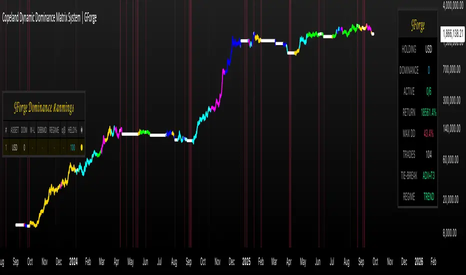
Copeland Dynamic Dominance Matrix System | GForgeCopeland Dynamic Dominance Matrix System | GForge - v1
---
📊 COMPREHENSIVE SYSTEM OVERVIEW
The GForge Dynamic BB% TrendSync System represents a revolutionary approach to algorithmic portfolio management, combining cutting-edge statistical analysis, momentum detection, and regime identification into a unified framework. This system processes up to 39 different cryptocurrency assets simultaneously, using advanced mathematical models to determine optimal capital allocation across dynamic market conditions.
Core Innovation: Multi-Dimensional Analysis
Unlike traditional single-asset indicators, this system operates on multiple analytical dimensions:
Momentum Analysis: Dual Bollinger Band Modified Deviation (DBBMD) calculations
Relative Strength: Comprehensive dominance matrix with head-to-head comparisons
Fundamental Screening: Alpha and Beta statistical filtering
Market Regime Detection: Five-component statistical testing framework
Portfolio Optimization: Dynamic weighting and allocation algorithms
Risk Management: Multi-layered protection and regime-based positioning
---
🔧 DETAILED COMPONENT BREAKDOWN
1. Dynamic Bollinger Band % Modified Deviation Engine (DBBMD)
The foundation of this system is an advanced oscillator that combines two independent Bollinger Band systems with asymmetric parameters to create unique momentum readings.
Technical Implementation:
[
// BB System 1: Fast-reacting with extended standard deviation
primary_bb1_ma_len = 40 // Shorter MA for responsiveness
primary_bb1_sd_len = 65 // Longer SD for stability
primary_bb1_mult = 1.0 // Standard deviation multiplier
// BB System 2: Complementary asymmetric design
primary_bb2_ma_len = 8 // Longer MA for trend following
primary_bb2_sd_len = 66 // Shorter SD for volatility sensitivity
primary_bb2_mult = 1.7 // Wider bands for reduced noise
Key Features:
Asymmetric Design: The intentional mismatch between MA and Standard Deviation periods creates unique oscillation characteristics that traditional Bollinger Bands cannot achieve
Percentage Scale: All readings are normalized to 0-100% scale for consistent interpretation across assets
Multiple Combination Modes:
BB1 Only: Fast/reactive system
BB2 Only: Smooth/stable system
Average: Balanced blend (recommended)
Both Required: Conservative (both must agree)
Either One: Aggressive (either can trigger)
Mean Deviation Filter: Additional volatility-based layer that measures the standard deviation of the DBBMD% itself, creating dynamic trigger bands
Signal Generation Logic:
// Primary thresholds
primary_long_threshold = 71 // DBBMD% level for bullish signals
primary_short_threshold = 33 // DBBMD% level for bearish signals
// Mean Deviation creates dynamic bands around these thresholds
upper_md_band = combined_bb + (md_mult * bb_std)
lower_md_band = combined_bb - (md_mult * bb_std)
// Signal triggers when DBBMD crosses these dynamic bands
long_signal = lower_md_band > long_threshold
short_signal = upper_md_band < short_threshold
For more information on this BB% indicator, find it here:
2. Revolutionary Dominance Matrix System
This is the system's most sophisticated innovation - a comprehensive framework that compares every asset against every other asset to determine relative strength hierarchies.
Mathematical Foundation:
The system constructs a mathematical matrix where each cell represents whether asset i dominates asset j:
// Core dominance matrix (39x39 for maximum assets)
var matrix dominance_matrix = matrix.new(39, 39, 0)
// For each qualifying asset pair (i,j):
for i = 0 to active_count - 1
for j = 0 to active_count - 1
if i != j
// Calculate price ratio BB% TrendSync for asset_i/asset_j
ratio_array = calculate_price_ratios(asset_i, asset_j)
ratio_dbbmd = calculate_dbbmd(ratio_array)
// Asset i dominates j if ratio is in uptrend
if ratio_dbbmd_state == 1
matrix.set(dominance_matrix, i, j, 1)
Copeland Scoring Algorithm:
Each asset receives a dominance score calculated as:
Dominance Score = Total Wins - Total Losses
// Calculate net dominance for each asset
for i = 0 to active_count - 1
wins = 0
losses = 0
for j = 0 to active_count - 1
if i != j
if matrix.get(dominance_matrix, i, j) == 1
wins += 1
else
losses += 1
copeland_score = wins - losses
array.set(dominance_scores, i, copeland_score)
Head-to-Head Analysis Process:
Ratio Construction: For each asset pair, calculate price_asset_A / price_asset_B
DBBMD Application: Apply the same DBBMD analysis to these ratios
Trend Determination: If ratio DBBMD shows uptrend, Asset A dominates Asset B
Matrix Population: Store dominance relationships in mathematical matrix
Score Calculation: Sum wins minus losses for final ranking
This creates a tournament-style ranking where each asset's strength is measured against all others, not just against a benchmark.
3. Advanced Alpha & Beta Filtering System
The system incorporates fundamental analysis through Capital Asset Pricing Model (CAPM) calculations to filter assets based on risk-adjusted performance.
Alpha Calculation (Excess Return Analysis):
// CAPM Alpha calculation
f_calc_alpha(asset_prices, benchmark_prices, alpha_length, beta_length, risk_free_rate) =>
// Calculate asset and benchmark returns
asset_returns = calculate_returns(asset_prices, alpha_length)
benchmark_returns = calculate_returns(benchmark_prices, alpha_length)
// Get beta for expected return calculation
beta = f_calc_beta(asset_prices, benchmark_prices, beta_length)
// Average returns over period
avg_asset_return = array_average(asset_returns) * 100
avg_benchmark_return = array_average(benchmark_returns) * 100
// Expected return using CAPM: E(R) = Beta * Market_Return + Risk_Free_Rate
expected_return = beta * avg_benchmark_return + risk_free_rate
// Alpha = Actual Return - Expected Return
alpha = avg_asset_return - expected_return
Beta Calculation (Volatility Relationship):
// Beta measures how much an asset moves relative to benchmark
f_calc_beta(asset_prices, benchmark_prices, length) =>
// Calculate return series for both assets
asset_returns =
benchmark_returns =
// Populate return arrays
for i = 0 to length - 1
asset_return = (current_price - previous_price) / previous_price
benchmark_return = (current_bench - previous_bench) / previous_bench
// Calculate covariance and variance
covariance = calculate_covariance(asset_returns, benchmark_returns)
benchmark_variance = calculate_variance(benchmark_returns)
// Beta = Covariance(Asset, Market) / Variance(Market)
beta = covariance / benchmark_variance
Filtering Applications:
Alpha Filter: Only includes assets with alpha above specified threshold (e.g., >0.5% monthly excess return)
Beta Filter: Screens for desired volatility characteristics (e.g., beta >1.0 for aggressive assets)
Combined Screening: Both filters must pass for asset qualification
Dynamic Thresholds: User-configurable parameters for different market conditions
4. Intelligent Tie-Breaking Resolution System
When multiple assets have identical dominance scores, the system employs sophisticated methods to determine final rankings.
Standard Tie-Breaking Hierarchy:
// Primary tie-breaking logic
if score_i == score_j // Tied dominance scores
// Level 1: Compare Beta values (higher beta wins)
beta_i = array.get(beta_values, i)
beta_j = array.get(beta_values, j)
if beta_j > beta_i
swap_positions(i, j)
else if beta_j == beta_i
// Level 2: Compare Alpha values (higher alpha wins)
alpha_i = array.get(alpha_values, i)
alpha_j = array.get(alpha_values, j)
if alpha_j > alpha_i
swap_positions(i, j)
Advanced Tie-Breaking (Head-to-Head Analysis):
For the top 3 performers, an enhanced tie-breaking mechanism analyzes direct head-to-head price ratio performance:
// Advanced tie-breaker for top performers
f_advanced_tiebreaker(asset1_idx, asset2_idx, lookback_period) =>
// Calculate price ratio over lookback period
ratio_history =
for k = 0 to lookback_period - 1
price_ratio = price_asset1 / price_asset2
array.push(ratio_history, price_ratio)
// Apply simplified trend analysis to ratio
current_ratio = array.get(ratio_history, 0)
average_ratio = calculate_average(ratio_history)
// Asset 1 wins if current ratio > average (trending up)
if current_ratio > average_ratio
return 1 // Asset 1 dominates
else
return -1 // Asset 2 dominates
5. Five-Component Aggregate Market Regime Filter
This sophisticated framework combines multiple statistical tests to determine whether market conditions favor trending strategies or require defensive positioning.
Component 1: Augmented Dickey-Fuller (ADF) Test
Tests for unit root presence to distinguish between trending and mean-reverting price series.
// Simplified ADF implementation
calculate_adf_statistic(price_series, lookback) =>
// Calculate first differences
differences =
for i = 0 to lookback - 2
diff = price_series - price_series
array.push(differences, diff)
// Statistical analysis of differences
mean_diff = calculate_mean(differences)
std_diff = calculate_standard_deviation(differences)
// ADF statistic approximation
adf_stat = mean_diff / std_diff
// Compare against threshold for trend determination
is_trending = adf_stat <= adf_threshold
Component 2: Directional Movement Index (DMI)
Classic Wilder indicator measuring trend strength through directional movement analysis.
// DMI calculation for trend strength
calculate_dmi_signal(high_data, low_data, close_data, period) =>
// Calculate directional movements
plus_dm_sum = 0.0
minus_dm_sum = 0.0
true_range_sum = 0.0
for i = 1 to period
// Directional movements
up_move = high_data - high_data
down_move = low_data - low_data
// Accumulate positive/negative movements
if up_move > down_move and up_move > 0
plus_dm_sum += up_move
if down_move > up_move and down_move > 0
minus_dm_sum += down_move
// True range calculation
true_range_sum += calculate_true_range(i)
// Calculate directional indicators
di_plus = 100 * plus_dm_sum / true_range_sum
di_minus = 100 * minus_dm_sum / true_range_sum
// ADX calculation
dx = 100 * math.abs(di_plus - di_minus) / (di_plus + di_minus)
adx = dx // Simplified for demonstration
// Trending if ADX above threshold
is_trending = adx > dmi_threshold
Component 3: KPSS Stationarity Test
Complementary test to ADF that examines stationarity around trend components.
// KPSS test implementation
calculate_kpss_statistic(price_series, lookback, significance_level) =>
// Calculate mean and variance
series_mean = calculate_mean(price_series, lookback)
series_variance = calculate_variance(price_series, lookback)
// Cumulative sum of deviations
cumulative_sum = 0.0
cumsum_squared_sum = 0.0
for i = 0 to lookback - 1
deviation = price_series - series_mean
cumulative_sum += deviation
cumsum_squared_sum += math.pow(cumulative_sum, 2)
// KPSS statistic
kpss_stat = cumsum_squared_sum / (lookback * lookback * series_variance)
// Compare against critical values
critical_value = significance_level == 0.01 ? 0.739 :
significance_level == 0.05 ? 0.463 : 0.347
is_trending = kpss_stat >= critical_value
Component 4: Choppiness Index
Measures market directionality using fractal dimension analysis of price movement.
// Choppiness Index calculation
calculate_choppiness(price_data, period) =>
// Find highest and lowest over period
highest = price_data
lowest = price_data
true_range_sum = 0.0
for i = 0 to period - 1
if price_data > highest
highest := price_data
if price_data < lowest
lowest := price_data
// Accumulate true range
if i > 0
true_range = calculate_true_range(price_data, i)
true_range_sum += true_range
// Choppiness calculation
range_high_low = highest - lowest
choppiness = 100 * math.log10(true_range_sum / range_high_low) / math.log10(period)
// Trending if choppiness below threshold (typically 61.8)
is_trending = choppiness < 61.8
Component 5: Hilbert Transform Analysis
Phase-based cycle detection and trend identification using mathematical signal processing.
// Hilbert Transform trend detection
calculate_hilbert_signal(price_data, smoothing_period, filter_period) =>
// Smooth the price data
smoothed_price = calculate_moving_average(price_data, smoothing_period)
// Calculate instantaneous phase components
// Simplified implementation for demonstration
instant_phase = smoothed_price
delayed_phase = calculate_moving_average(price_data, filter_period)
// Compare instantaneous vs delayed signals
phase_difference = instant_phase - delayed_phase
// Trending if instantaneous leads delayed
is_trending = phase_difference > 0
Aggregate Regime Determination:
// Combine all five components
regime_calculation() =>
trending_count = 0
total_components = 0
// Test each enabled component
if enable_adf and adf_signal == 1
trending_count += 1
if enable_adf
total_components += 1
// Repeat for all five components...
// Calculate trending proportion
trending_proportion = trending_count / total_components
// Market is trending if proportion above threshold
regime_allows_trading = trending_proportion >= regime_threshold
The system only allows asset positions when the specified percentage of components indicate trending conditions. During choppy or mean-reverting periods, the system automatically positions in USD to preserve capital.
6. Dynamic Portfolio Weighting Framework
Six sophisticated allocation methodologies provide flexibility for different market conditions and risk preferences.
Weighting Method Implementations:
1. Equal Weight Distribution:
// Simple equal allocation
if weighting_mode == "Equal Weight"
weight_per_asset = 1.0 / selection_count
for i = 0 to selection_count - 1
array.push(weights, weight_per_asset)
2. Linear Dominance Scaling:
// Linear scaling based on dominance scores
if weighting_mode == "Linear Dominance"
// Normalize scores to 0-1 range
min_score = array.min(dominance_scores)
max_score = array.max(dominance_scores)
score_range = max_score - min_score
total_weight = 0.0
for i = 0 to selection_count - 1
score = array.get(dominance_scores, i)
normalized = (score - min_score) / score_range
weight = 1.0 + normalized * concentration_factor
array.push(weights, weight)
total_weight += weight
// Normalize to sum to 1.0
for i = 0 to selection_count - 1
current_weight = array.get(weights, i)
array.set(weights, i, current_weight / total_weight)
3. Conviction Score (Exponential):
// Exponential scaling for high conviction
if weighting_mode == "Conviction Score"
// Combine dominance score with DBBMD strength
conviction_scores =
for i = 0 to selection_count - 1
dominance = array.get(dominance_scores, i)
dbbmd_strength = array.get(dbbmd_values, i)
conviction = dominance + (dbbmd_strength - 50) / 25
array.push(conviction_scores, conviction)
// Exponential weighting
total_weight = 0.0
for i = 0 to selection_count - 1
conviction = array.get(conviction_scores, i)
normalized = normalize_score(conviction)
weight = math.pow(1 + normalized, concentration_factor)
array.push(weights, weight)
total_weight += weight
// Final normalization
normalize_weights(weights, total_weight)
Advanced Features:
Minimum Position Constraint: Prevents dust allocations below specified threshold
Concentration Factor: Adjustable parameter controlling weight distribution aggressiveness
Dominance Boost: Extra weight for assets exceeding specified dominance thresholds
Dynamic Rebalancing: Automatic weight recalculation on portfolio changes
7. Intelligent USD Management System
The system treats USD as a competing asset with its own dominance score, enabling sophisticated cash management.
USD Scoring Methodologies:
Smart Competition Mode (Recommended):
f_calculate_smart_usd_dominance() =>
usd_wins = 0
// USD beats assets in downtrends or weak uptrends
for i = 0 to active_count - 1
asset_state = get_asset_state(i)
asset_dbbmd = get_asset_dbbmd(i)
// USD dominates shorts and weak longs
if asset_state == -1 or (asset_state == 1 and asset_dbbmd < long_threshold)
usd_wins += 1
// Calculate Copeland-style score
base_score = usd_wins - (active_count - usd_wins)
// Boost during weak market conditions
qualified_assets = count_qualified_long_assets()
if qualified_assets <= active_count * 0.2
base_score := math.round(base_score * usd_boost_factor)
base_score
Auto Short Count Mode:
// USD dominance based on number of bearish assets
usd_dominance = count_assets_in_short_state()
// Apply boost during low activity
if qualified_long_count <= active_count * 0.2
usd_dominance := usd_dominance * usd_boost_factor
Regime-Based USD Positioning:
When the five-component regime filter indicates unfavorable conditions, the system automatically overrides all asset signals and positions 100% in USD, protecting capital during choppy markets.
8. Multi-Asset Infrastructure & Data Management
The system maintains comprehensive data structures for up to 39 assets simultaneously.
Data Collection Framework:
// Full OHLC data matrices (200 bars depth for performance)
var matrix open_data = matrix.new(39, 200, na)
var matrix high_data = matrix.new(39, 200, na)
var matrix low_data = matrix.new(39, 200, na)
var matrix close_data = matrix.new(39, 200, na)
// Real-time data collection
if barstate.isconfirmed
for i = 0 to active_count - 1
ticker = array.get(assets, i)
= request.security(ticker, timeframe.period,
[open , high , low , close ],
lookahead=barmerge.lookahead_off)
// Store in matrices with proper shifting
matrix.set(open_data, i, 0, nz(o, 0))
matrix.set(high_data, i, 0, nz(h, 0))
matrix.set(low_data, i, 0, nz(l, 0))
matrix.set(close_data, i, 0, nz(c, 0))
Asset Configuration:
The system comes pre-configured with 39 major cryptocurrency pairs across multiple exchanges:
Major Pairs: BTC, ETH, XRP, SOL, DOGE, ADA, etc.
Exchange Coverage: Binance, KuCoin, MEXC for optimal liquidity
Configurable Count: Users can activate 2-39 assets based on preferences
Custom Tickers: All asset selections are user-modifiable
---
⚙️ COMPREHENSIVE CONFIGURATION GUIDE
Portfolio Management Settings
Maximum Portfolio Size (1-10):
Conservative (1-2): High concentration, captures strong trends
Balanced (3-5): Moderate diversification with trend focus
Diversified (6-10): Lower concentration, broader market exposure
Dominance Clarity Threshold (0.1-1.0):
Low (0.1-0.4): Prefers diversification, holds multiple assets frequently
Medium (0.5-0.7): Balanced approach, context-dependent allocation
High (0.8-1.0): Concentration-focused, single asset preference
Signal Generation Parameters
DBBMD Thresholds:
// Standard configuration
primary_long_threshold = 71 // Conservative: 75+, Aggressive: 65-70
primary_short_threshold = 33 // Conservative: 25-30, Aggressive: 35-40
// BB System parameters
bb1_ma_len = 40 // Fast system: 20-50
bb1_sd_len = 65 // Stability: 50-80
bb2_ma_len = 8 // Trend: 60-100
bb2_sd_len = 66 // Sensitivity: 10-20
Risk Management Configuration
Alpha/Beta Filters:
Alpha Threshold: 0.0-2.0% (higher = more selective)
Beta Threshold: 0.5-2.0 (1.0+ for aggressive assets)
Calculation Periods: 20-50 bars (longer = more stable)
Regime Filter Settings:
Trending Threshold: 0.3-0.8 (higher = stricter trend requirements)
Component Lookbacks: 30-100 bars (balance responsiveness vs stability)
Enable/Disable: Individual component control for customization
---
📊 PERFORMANCE TRACKING & VISUALIZATION
Real-Time Dashboard Features
The compact dashboard provides essential information:
Current Holdings: Asset names and allocation percentages
Dominance Score: Current position's relative strength ranking
Active Assets: Qualified long signals vs total asset count
Returns: Total portfolio performance percentage
Maximum Drawdown: Peak-to-trough decline measurement
Trade Count: Total portfolio transitions executed
Regime Status: Current market condition assessment
Comprehensive Ranking Table
The left-side table displays detailed asset analysis:
Ranking Position: Numerical order by dominance score
Asset Symbol: Clean ticker identification with color coding
Dominance Score: Net wins minus losses in head-to-head comparisons
Win-Loss Record: Detailed breakdown of dominance relationships
DBBMD Reading: Current momentum percentage with threshold highlighting
Alpha/Beta Values: Fundamental analysis metrics when filters enabled
Portfolio Weight: Current allocation percentage in signal portfolio
Execution Status: Visual indicator of actual holdings vs signals
Visual Enhancement Features
Color-Coded Assets: 39 distinct colors for easy identification
Regime Background: Red tinting during unfavorable market conditions
Dynamic Equity Curve: Portfolio value plotted with position-based coloring
Status Indicators: Symbols showing execution vs signal states
---
🔍 ADVANCED TECHNICAL FEATURES
State Persistence System
The system maintains asset states across bars to prevent excessive switching:
// State tracking for each asset and ratio combination
var array asset_states = array.new(1560, 0) // 39 * 40 ratios
// State changes only occur on confirmed threshold breaks
if long_crossover and current_state != 1
current_state := 1
array.set(asset_states, asset_index, 1)
else if short_crossover and current_state != -1
current_state := -1
array.set(asset_states, asset_index, -1)
Transaction Cost Integration
Realistic modeling of trading expenses:
// Transaction cost calculation
transaction_fee = 0.4 // Default 0.4% (fees + slippage)
// Applied on portfolio transitions
if should_execute_transition
was_holding_assets = check_current_holdings()
will_hold_assets = check_new_signals()
// Charge fees for meaningful transitions
if transaction_fee > 0 and (was_holding_assets or will_hold_assets)
fee_amount = equity * (transaction_fee / 100)
equity -= fee_amount
total_fees += fee_amount
Dynamic Memory Management
Optimized data structures for performance:
200-Bar History: Sufficient for calculations while maintaining speed
Matrix Operations: Efficient storage and retrieval of multi-asset data
Array Recycling: Memory-conscious data handling for long-running backtests
Conditional Calculations: Skip unnecessary computations during initialization
12H 30 assets portfolio
---
🚨 SYSTEM LIMITATIONS & TESTING STATUS
CURRENT DEVELOPMENT PHASE: ACTIVE TESTING & OPTIMIZATION
This system represents cutting-edge algorithmic trading technology but remains in continuous development. Key considerations:
Known Limitations:
Requires significant computational resources for 39-asset analysis
Performance varies significantly across different market conditions
Complex parameter interactions may require extensive optimization
Slippage and liquidity constraints not fully modeled for all assets
No consideration for market impact in large position sizes
Areas Under Active Development:
Enhanced regime detection algorithms
Improved transaction cost modeling
Additional portfolio weighting methodologies
Machine learning integration for parameter optimization
Cross-timeframe analysis capabilities
---
🔒 ANTI-REPAINTING ARCHITECTURE & LIVE TRADING READINESS
One of the most critical aspects of any trading system is ensuring that signals and calculations are based on confirmed, historical data rather than current bar information that can change throughout the trading session. This system implements comprehensive anti-repainting measures to ensure 100% reliability for live trading .
The Repainting Problem in Trading Systems
Repainting occurs when an indicator uses current, unconfirmed bar data in its calculations, causing:
False Historical Signals: Backtests appear better than reality because calculations change as bars develop
Live Trading Failures: Signals that looked profitable in testing fail when deployed in real markets
Inconsistent Results: Different results when running the same indicator at different times during a trading session
Misleading Performance: Inflated win rates and returns that cannot be replicated in practice
GForge Anti-Repainting Implementation
This system eliminates repainting through multiple technical safeguards:
1. Historical Data Usage for All Calculations
// CRITICAL: All calculations use PREVIOUS bar data (note the offset)
= request.security(ticker, timeframe.period,
[open , high , low , close , close],
lookahead=barmerge.lookahead_off)
// Store confirmed previous bar OHLC for calculations
matrix.set(open_data, i, 0, nz(o1, 0)) // Previous bar open
matrix.set(high_data, i, 0, nz(h1, 0)) // Previous bar high
matrix.set(low_data, i, 0, nz(l1, 0)) // Previous bar low
matrix.set(close_data, i, 0, nz(c1, 0)) // Previous bar close
// Current bar close only for visualization
matrix.set(current_prices, i, 0, nz(c0, 0)) // Live price display
2. Confirmed Bar State Processing
// Only process data when bars are confirmed and closed
if barstate.isconfirmed
// All signal generation and portfolio decisions occur here
// using only historical, unchanging data
// Shift historical data arrays
for i = 0 to active_count - 1
for bar = math.min(data_bars, 199) to 1
// Move confirmed data through historical matrices
old_data = matrix.get(close_data, i, bar - 1)
matrix.set(close_data, i, bar, old_data)
// Process new confirmed bar data
calculate_all_signals_and_dominance()
3. Lookahead Prevention
// Explicit lookahead prevention in all security calls
request.security(ticker, timeframe.period, expression,
lookahead=barmerge.lookahead_off)
// This ensures no future data can influence current calculations
// Essential for maintaining signal integrity across all timeframes
4. State Persistence with Historical Validation
// Asset states only change based on confirmed threshold breaks
// using historical data that cannot change
var array asset_states = array.new(1560, 0)
// State changes use only confirmed, previous bar calculations
if barstate.isconfirmed
=
f_calculate_enhanced_dbbmd(confirmed_price_array, ...)
// Only update states after bar confirmation
if long_crossover_confirmed and current_state != 1
current_state := 1
array.set(asset_states, asset_index, 1)
Live Trading vs. Backtesting Consistency
The system's architecture ensures identical behavior in both environments:
Backtesting Mode:
Uses historical offset data for all calculations
Processes confirmed bars with `barstate.isconfirmed`
Maintains identical signal generation logic
No access to future information
Live Trading Mode:
Uses same historical offset data structure
Waits for bar confirmation before signal updates
Identical mathematical calculations and thresholds
Real-time price display without affecting signals
Technical Implementation Details
Data Collection Timing
// Example of proper data collection timing
if barstate.isconfirmed // Wait for bar to close
// Collect PREVIOUS bar's confirmed OHLC data
for i = 0 to active_count - 1
ticker = array.get(assets, i)
// Get confirmed previous bar data (note offset)
=
request.security(ticker, timeframe.period,
[open , high , low , close , close],
lookahead=barmerge.lookahead_off)
// ALL calculations use prev_* values
// current_close only for real-time display
portfolio_calculations_use_previous_bar_data()
Signal Generation Process
// Signal generation workflow (simplified)
if barstate.isconfirmed and data_bars >= minimum_required_bars
// Step 1: Calculate DBBMD using historical price arrays
for i = 0 to active_count - 1
historical_prices = get_confirmed_price_history(i) // Uses offset data
= calculate_dbbmd(historical_prices)
update_asset_state(i, state)
// Step 2: Build dominance matrix using confirmed data
calculate_dominance_relationships() // All historical data
// Step 3: Generate portfolio signals
new_portfolio = generate_target_portfolio() // Based on confirmed calculations
// Step 4: Compare with previous signals for changes
if portfolio_signals_changed()
execute_portfolio_transition()
Verification Methods for Users
Users can verify the anti-repainting behavior through several methods:
1. Historical Replay Test
Run the indicator on historical data
Note signal timing and portfolio changes
Replay the same period - signals should be identical
No retroactive changes in historical signals
2. Intraday Consistency Check
Load indicator during active trading session
Observe that previous day's signals remain unchanged
Only current day's final bar should show potential signal changes
Refresh indicator - historical signals should be identical
Live Trading Deployment Considerations
Data Quality Assurance
Exchange Connectivity: Ensure reliable data feeds for all 39 assets
Missing Data Handling: System includes safeguards for data gaps
Price Validation: Automatic filtering of obvious price errors
Timeframe Synchronization: All assets synchronized to same bar timing
Performance Impact of Anti-Repainting Measures
The robust anti-repainting implementation requires additional computational resources:
Memory Usage: 200-bar historical data storage for 39 assets
Processing Delay: Signals update only after bar confirmation
Calculation Overhead: Multiple historical data validations
Alert Timing: Slight delay compared to current-bar indicators
However, these trade-offs are essential for reliable live trading performance and accurate backtesting results.
Critical: Equity Curve Anti-Repainting Architecture
The most sophisticated aspect of this system's anti-repainting design is the temporal separation between signal generation and performance calculation . This creates a realistic trading simulation that perfectly matches live trading execution.
The Timing Sequence
// STEP 1: Store what we HELD during the current bar (for performance calc)
if barstate.isconfirmed
// Record positions that were active during this bar
array.clear(held_portfolio)
array.clear(held_weights)
for i = 0 to array.size(execution_portfolio) - 1
array.push(held_portfolio, array.get(execution_portfolio, i))
array.push(held_weights, array.get(execution_weights, i))
// STEP 2: Calculate performance based on what we HELD
portfolio_return = 0.0
for i = 0 to array.size(held_portfolio) - 1
held_asset = array.get(held_portfolio, i)
held_weight = array.get(held_weights, i)
// Performance from current_price vs reference_price
// This is what we ACTUALLY earned during this bar
if held_asset != "USD"
current_price = get_current_price(held_asset) // End of bar
reference_price = get_reference_price(held_asset) // Start of bar
asset_return = (current_price - reference_price) / reference_price
portfolio_return += asset_return * held_weight
// STEP 3: Apply return to equity (realistic timing)
equity := equity * (1 + portfolio_return)
// STEP 4: Generate NEW signals for NEXT period (using confirmed data)
= f_generate_target_portfolio()
// STEP 5: Execute transitions if signals changed
if signal_changed
// Update execution_portfolio for NEXT bar
array.clear(execution_portfolio)
array.clear(execution_weights)
for i = 0 to array.size(new_signal_portfolio) - 1
array.push(execution_portfolio, array.get(new_signal_portfolio, i))
array.push(execution_weights, array.get(new_signal_weights, i))
Why This Prevents Equity Curve Repainting
Performance Attribution: Returns are calculated based on positions that were **actually held** during each bar, not future signals
Signal Timing: New signals are generated **after** performance calculation, affecting only **future** bars
Realistic Execution: Mimics real trading where you earn returns on current positions while planning future moves
No Retroactive Changes: Once a bar closes, its performance contribution to equity is permanent and unchangeable
The One-Bar Offset Mechanism
This system implements a critical one-bar timing offset:
// Bar N: Performance Calculation
// ================================
// 1. Calculate returns on positions held during Bar N
// 2. Update equity based on actual holdings during Bar N
// 3. Plot equity point for Bar N (based on what we HELD)
// Bar N: Signal Generation
// ========================
// 4. Generate signals for Bar N+1 (using confirmed Bar N data)
// 5. Send alerts for what will be held during Bar N+1
// 6. Update execution_portfolio for Bar N+1
// Bar N+1: The Cycle Continues
// =============================
// 1. Performance calculated on positions from Bar N signals
// 2. New signals generated for Bar N+2
Alert System Timing
The alert system reflects this sophisticated timing:
Transaction Cost Realism
Even transaction costs follow realistic timing:
// Fees applied when transitioning between different portfolios
if should_execute_transition
// Charge fees BEFORE taking new positions (realistic timing)
if transaction_fee > 0
fee_amount = equity * (transaction_fee / 100)
equity -= fee_amount // Immediate cost impact
total_fees += fee_amount
// THEN update to new portfolio
update_execution_portfolio(new_signals)
transitions += 1
// Fees reduce equity immediately, affecting all future calculations
// This matches real trading where fees are deducted upon execution
LIVE TRADING CERTIFICATION:
This system has been specifically designed and tested for live trading deployment. The comprehensive anti-repainting measures ensure that:
Backtesting results accurately represent real trading potential
Signals are generated using only confirmed, historical data
No retroactive changes can occur to previously generated signals
Portfolio transitions are based on reliable, unchanging calculations
Performance metrics reflect realistic trading outcomes including proper timing
Users can deploy this system with confidence that live trading results will closely match backtesting performance, subject to normal market execution factors such as slippage and liquidity.
---
⚡ ALERT SYSTEM & AUTOMATION
The system provides comprehensive alerting for automation and monitoring:
Available Alert Conditions
Portfolio Signal Change: Triggered when new portfolio composition is generated
Regime Override Active: Alerts when market regime forces USD positioning
Individual Asset Signals: Can be configured for specific asset transitions
Performance Thresholds: Drawdown or return-based notifications
---
📈 BACKTESTING & PERFORMANCE ANALYSIS
8 Comprehensive Metrics Tracking
The system maintains detailed performance statistics:
Equity Curve: Real-time portfolio value progression
Returns Calculation: Total and annualized performance metrics
Drawdown Analysis: Peak-to-trough decline measurements
Transaction Counting: Portfolio transition frequency
Fee Tracking: Cumulative transaction cost impact
Win Rate Analysis: Success rate of position changes
Backtesting Configuration
// Backtesting parameters
initial_capital = 10000.0 // Starting capital
use_custom_start = true // Enable specific start date
custom_start = timestamp("2023-09-01") // Backtest beginning
transaction_fee = 0.4 // Combined fees and slippage %
// Performance calculation
total_return = (equity - initial_capital) / initial_capital * 100
current_drawdown = (peak_equity - equity) / peak_equity * 100
---
🔧 TROUBLESHOOTING & OPTIMIZATION
Common Configuration Issues
Insufficient Data: Ensure 100+ bars available before start date
[*} Not Compiling: Go on an asset's price chart with 2 or 3 years of data to
make the system compile or just simply reapply the indicator again
Too Many Assets: Reduce active count if experiencing timeouts
Regime Filter Too Strict: Lower trending threshold if always in USD
Excessive Switching: Increase MD multiplier or adjust thresholds
---
💡 USER FEEDBACK & ENHANCEMENT REQUESTS
The continuous evolution of this system depends heavily on user experience and community feedback. Your insights will help motivate me for new improvements and new feature developments.
---
⚖️ FINAL COMPREHENSIVE RISK DISCLAIMER
TRADING INVOLVES SUBSTANTIAL RISK OF LOSS
This indicator is a sophisticated analytical tool designed for educational and research purposes. Important warnings and considerations:
System Limitations:
No algorithmic system can guarantee profitable outcomes
Complex systems may fail in unexpected ways during extreme market events
Historical backtesting does not account for all real-world trading challenges
Slippage, liquidity constraints, and market impact can significantly affect results
System parameters require careful optimization and ongoing monitoring
The creator and distributor of this indicator assume no liability for any financial losses, system failures, or adverse outcomes resulting from its use. This tool is provided "as is" without any warranties, express or implied.
By using this indicator, you acknowledge that you have read, understood, and agreed to assume all risks associated with algorithmic trading and cryptocurrency investments.
Mikula's Master 360° Square of 12Mikula’s Master 360° Square of 12
An educational W. D. Gann study indicator for price and time. Anchor a compact Square of 12 table to a start point you choose. Begin from a bar’s High or Low (or set a manual start price). From that anchor you can progress or regress the table to study how price steps through cycles in either direction.
What you’re looking at :
Zodiac rail (far left): the twelve signs.
Degree rail: 24 rows in 15° steps from 15° up to 360°/0°.
Transit rail and Natal rail: track one planet per rail. Each planet is placed at its current row (℞ shown when retrograde). As longitude advances, the planet climbs bottom → top, then wraps to the bottom at the next sign; during retrograde it steps downward.
Hover a planet’s cell to see a tooltip with its exact longitude and sign (e.g., 152.4° ♌︎). The linked price cell in the grid moves with the planet’s row so you can follow a planet’s path through the zodiac as a path through price.
Price grid (right): the 12×24 Square of 12. Each column is a cycle; cells are stepped price levels from your start price using your increment.
Bottom rail: shows the current square number and labels the twelve columns in that square.
How the square is read
The square always begins at the bottom left. Read each column bottom → top. At the top, return to the bottom of the next column and read up again. One square contains twelve cycles. Because the anchor can be a High or a Low, you can progress the table upward from the anchor or regress it downward while keeping the same bottom-to-top reading order.
Iterate Square (shifting)
Iterate Square shifts the entire 12×24 grid to the next set of twelve cycles.
Square 1 shows cycles 1–12; Square 2 shows 13–24; Square 3 shows 25–36, etc.
Visibility rules
Pivot cells are table-bound. If you shift the square beyond those prices, their highlights won’t appear in the table.
A/B levels and Transit/Natal planetary lines are chart overlays and can remain visible on the table as you shift the square.
Quick use
Choose an anchor (date/time + High/Low) or enable a manual start price .
Set the increment. If you anchored with a Low and want the table to step downward from there, use a negative value.
Optional: pick Transit and Natal planets (one per rail), toggle their plots, and hover their cells for longitude/sign.
Optional: turn on A/B levels to display repeating bands from the start price.
Optional: enable swing pivots to tint matching cells after the anchor.
Use Iterate Square to shift to later squares of twelve cycles.
Examples
These are exploratory examples to spark ideas:
Overview layout (zodiac & degree rails, Transit/Natal rails, price grid)
A-levels plotted, pivots tinted on the table, real-time price highlighted
Drawing angles from the anchor using price & time read from the table
Using a TradingView Gann box along the A-levels to study reactions
Attribution & originality
This script is an original implementation (no external code copied). Conceptual credit to Patrick Mikula, whose discussion of the Master 360° Square of 12 inspired this study’s presentation.
Further reading (neutral pointers)
Patrick Mikula, Gann’s Scientific Methods Unveiled, Vol. 2, “W. D. Gann’s Use of the Circle Chart.”
W. D. Gann’s Original Commodity Course (as provided by WDGAN.com).
No affiliation implied.
License CC BY-NC-SA 4.0 (non-commercial; please attribute @Javonnii and link the original).
Dependency AstroLib by @BarefootJoey
Disclaimer Educational use only; not financial advice.

Quantum Yield MatrixQuantum Yield Matrix is a sophisticated Pine Script™ v6 indicator designed to empower traders with a dynamic visualization of compound returns across global markets. It generates a customizable table showcasing daily percentage changes, cumulative compound returns, and performance differentials for a user-selected index and up to 10 stocks within a defined date range. The table automatically updates when the date range is modified, ensuring seamless flexibility for analysis. Ideal for portfolio evaluation, benchmark comparisons, and multi-exchange tracking, this tool operates independently of external data sources.
Key Features
Multi-Exchange Support: Integrates data from major exchanges, including BIST (Turkey), NYSE and NASDAQ (USA), SSE (China Shanghai Composite), XETR (Germany DAX), NSE (India NIFTY), and TVC (Japan Nikkei and other indices). Users select a single exchange per analysis, with automatic prefixing for accurate symbol resolution (e.g., NASDAQ:NDX).
Performance Metrics: Computes daily returns ((close - previous close) / previous close), aggregates compound returns over the period, and provides:Total return percentages.
Stock-versus-index performance differences (e.g., alpha insights).
A bottom summary comparing the watchlist’s average return to the index.
Visual Table Design: Features a color-coded table (green for positive returns, red for negative, gray for totals) with date headers for intuitive readability. Missing data is elegantly handled with "No Data" in gray cells, ensuring robust calculations.
Dynamic Customization: Allows full adjustment of exchange, index symbol (e.g., NDX for NASDAQ), stock symbols (e.g., AAPL, TSLA), and date range. The table dynamically recalculates when the date range changes, making it perfect for backtesting or forward-looking analysis.
Purpose and BenefitsQuantum Yield Matrix delivers a quantum leap in yield analysis by organizing complex return data into a clear, matrix-like table. It simplifies portfolio performance evaluation against benchmarks, highlighting outperforming assets at a glance. Whether assessing a NASDAQ tech portfolio against NDX or exploring emerging market stocks, this tool saves time, enhances decision-making, and fosters cross-market awareness for diversified strategies in today’s interconnected global economy.
How It Works
Setup: In the indicator settings, select an exchange (default: NASDAQ), input the index symbol (e.g., NDX), and up to 10 stock symbols (defaults: AAPL, TSLA, MSFT, etc.). Define the analysis period with start and end dates. Adjusting the date range instantly updates the table.
Data Retrieval: Leverages TradingView’s request.security function to fetch daily closing prices for each symbol, respecting the chosen exchange prefix (e.g., "NASDAQ:NDX").
Calculations:Daily returns are calculated as percentage changes.
Compound returns accumulate multiplicatively (starting from 1.0, multiplied by (1 + daily return)).
Comparisons subtract index returns from each stock’s total, with averages summarized at the bottom.
Rendering: Constructs a detailed table at the top-center of the chart and a summary table at the bottom. The script aligns with the chart’s timeframe but aggregates data to daily ("D") for consistency.
Edge Cases: If data is unavailable (e.g., due to exchange-specific holidays), cells display "No Data," preserving the integrity of compound return calculations.
Important Usage Note: For optimal results, set your chart symbol to match the analyzed exchange, such as NASDAQ:NDX for US data. The indicator relies on the chart’s bars, so mismatched symbols (e.g., a BIST symbol for US data) may skip non-trading days (e.g., July 15, a Turkish holiday).
Use daily or higher timeframes for best performance.
Disclaimer
This indicator is provided for educational and informational purposes only and does not constitute financial, investment, or trading advice. Past performance is not indicative of future results, and all trading involves risk of loss. Users are solely responsible for their decisions. The script is original, uses only built-in Pine Script functions, and complies with TradingView’s publishing rules—no external libraries, exaggerated claims, or guarantees are implied. Always verify data accuracy and consult professionals before acting on insights.
Feedback is welcome—feel free to fork and enhance!

Quantum Harmonic Oscillator Overlay🧪 Quantum Harmonic Oscillator Overlay
A visual model of price behavior using quantum harmonic oscillation principles
📜 Indicator Overview
The Quantum Harmonic Oscillator Overlay applies concepts from both classical physics (harmonic motion) and quantum mechanics (energy states) to model and visualize how price orbits around a central trend line. It overlays a Linear Regression line (representing the “mean position” or ground state of price) and calculates surrounding energy levels (σ-zones) akin to quantum shells that price can "jump" between.
This indicator is particularly useful for visualizing mean reversion, volatility compression/expansion, and momentum-driven price breakthroughs.
🧠 Core Concepts
Linear Regression Line (LSR): This is the calculated center of gravity or equilibrium path of price over a user-defined period. Think of it like the lowest energy state or central axis around which price vibrates.
Standard Deviation Zones (σ-levels):
1σ: The majority of normal price activity; within this range, price tends to fluctuate if in balance.
2σ: Indicates volatility or possible breakout pressure.
3σ: Represents extreme movement — a phase shift in energy, potentially leading to reversal or continuation with higher momentum.
Quantum Analogy: Just like in a quantum harmonic oscillator, particles (here, prices) move probabilistically between discrete energy states. The further the price moves from the center, the more "energy" (momentum, volume, volatility) is implied.
⚙️ Input Parameters
Setting Description
Linear Regression Length The number of bars used to calculate the regression trend (default 100). Affects the central path and responsiveness.
σ Multipliers (1σ, 2σ, 3σ) Determine how far each band is from the regression line. Adjusting these can highlight different price behaviors.
Show Energy Level Zones Toggle visibility of the colored bands around the regression line.
Show LSR Center Line Toggles visibility of the white Linear Regression line itself.
🎨 Visual Components
Color Zone Interpretation
✅ Green ±1σ Normal oscillation / mean reversion area. Ideal for range-bound strategies.
🟧 Orange ±2σ Warning zone; price may be gaining momentum or volatility.
🔴 Red ±3σ High-momentum state or anomaly. These regions may imply trend exhaustion, reversals, or breakouts.
White Line: The LSR — the average trajectory of the price movement.
Pink Dots: Appear when price exceeds Zone 3 (outside ±3σ) — a signal of extreme behavior or a possible regime shift.
📈 How to Use This Indicator
1. Detect Overextensions
When price touches or breaches the 3σ zone, it is likely overextended. This can be used to anticipate potential snapbacks or strong breakout trends.
2. Identify Mean Reversion Trades
If price exits the 2σ or 3σ zones and returns toward the center line, this signals a likely mean reversion setup.
3. Volatility Compression or Expansion
Flat zones between σ levels suggest calm markets; widening bands suggest expanding volatility.
4. Use with Confirmation Tools
Combine with momentum oscillators (MACD, RSI) or volume-based signals to confirm reversals or continuation outside Zone 3.
🔮 Philosophical Note
This indicator embodies the metaphor that the market behaves like a quantum oscillator — price particles exist in a probabilistic field and jump between discrete zones of volatility and energy. Tracking these transitions allows the trader to see price behavior as rhythmic, wave-like, and multidimensional rather than purely linear.

Trailing Monster StrategyTrailing Monster Strategy
This is an experimental trend-following strategy that incorporates a custom adaptive moving average (PKAMA), RSI-based momentum filtering, and dynamic trailing stop-loss logic. It is designed for educational and research purposes only, and may require further optimization or risk management considerations prior to live deployment.
Strategy Logic
The strategy attempts to participate in sustained price trends by combining:
- A Power Kaufman Adaptive Moving Average (PKAMA) for dynamic trend detection,
- RSI and Simple Moving Average (SMA) filters for market condition confirmation,
- A delayed trailing stop-loss to manage exits once a trade is in profit.
Entry Conditions
Long Entry:
- RSI exceeds the overbought threshold (default: 70),
- Price is trading above the 200-period SMA,
- PKAMA slope is positive (indicating upward momentum),
- A minimum number of bars have passed since the last entry.
Short Entry:
- RSI falls below the oversold threshold (default: 30),
- Price is trading below the 200-period SMA,
- PKAMA slope is negative (indicating downward momentum),
-A minimum number of bars have passed since the last entry.
Exit Conditions
- A trailing stop-loss is applied once the position has been open for a user-defined number of bars.
- The trailing distance is calculated as a fixed percentage of the average entry price.
Technical Notes
This script implements a custom version of the Power Kaufman Adaptive Moving Average (PKAMA), conceptually inspired by alexgrover’s public implementation on TradingView .
Unlike traditional moving averages, PKAMA dynamically adjusts its responsiveness based on recent market volatility, allowing it to better capture trend changes in fast-moving assets like altcoins.
Disclaimer
This strategy is provided for educational purposes only.
It is not financial advice, and no guarantee of profitability is implied.
Always conduct thorough backtesting and forward testing before using any strategy in a live environment.
Adjust inputs based on your individual risk tolerance, asset class, and trading style.
Feedback is encouraged. You are welcome to fork and modify this script to suit your own preferences and market approach.
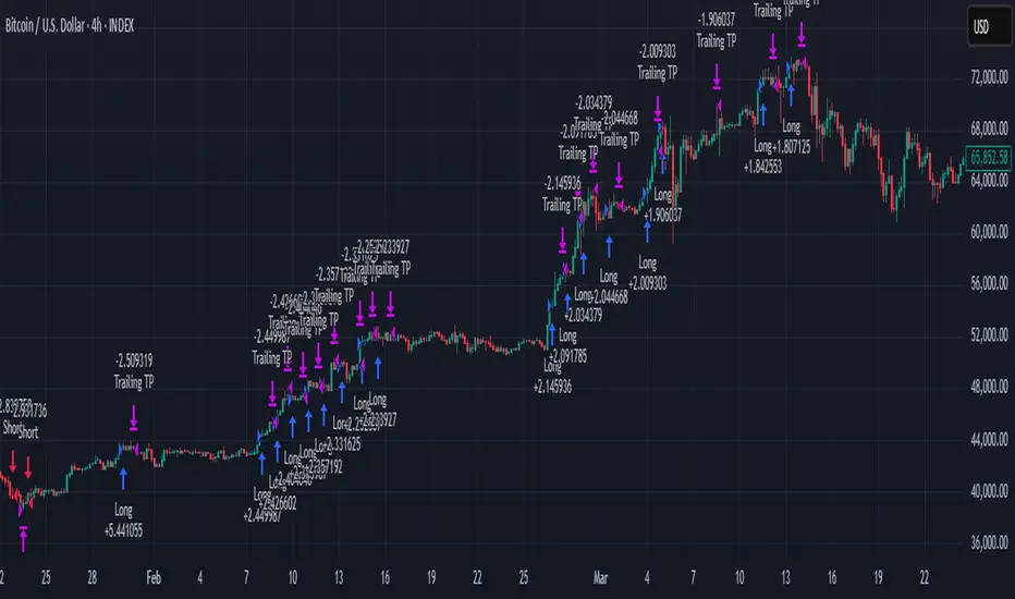
Enhanced Fuzzy SMA Analyzer (Multi-Output Proxy) [FibonacciFlux]EFzSMA: Decode Trend Quality, Conviction & Risk Beyond Simple Averages
Stop Relying on Lagging Averages Alone. Gain a Multi-Dimensional Edge.
The Challenge: Simple Moving Averages (SMAs) tell you where the price was , but they fail to capture the true quality, conviction, and sustainability of a trend. Relying solely on price crossing an average often leads to chasing weak moves, getting caught in choppy markets, or missing critical signs of trend exhaustion. Advanced traders need a more sophisticated lens to navigate complex market dynamics.
The Solution: Enhanced Fuzzy SMA Analyzer (EFzSMA)
EFzSMA is engineered to address these limitations head-on. It moves beyond simple price-average comparisons by employing a sophisticated Fuzzy Inference System (FIS) that intelligently integrates multiple critical market factors:
Price deviation from the SMA ( adaptively normalized for market volatility)
Momentum (Rate of Change - ROC)
Market Sentiment/Overheat (Relative Strength Index - RSI)
Market Volatility Context (Average True Range - ATR, optional)
Volume Dynamics (Volume relative to its MA, optional)
Instead of just a line on a chart, EFzSMA delivers a multi-dimensional assessment designed to give you deeper insights and a quantifiable edge.
Why EFzSMA? Gain Deeper Market Insights
EFzSMA empowers you to make more informed decisions by providing insights that simple averages cannot:
Assess True Trend Quality, Not Just Location: Is the price above the SMA simply because of a temporary spike, or is it supported by strong momentum, confirming volume, and stable volatility? EFzSMA's core fuzzyTrendScore (-1 to +1) evaluates the health of the trend, helping you distinguish robust moves from noise.
Quantify Signal Conviction: How reliable is the current trend signal? The Conviction Proxy (0 to 1) measures the internal consistency among the different market factors analyzed by the FIS. High conviction suggests factors are aligned, boosting confidence in the trend signal. Low conviction warns of conflicting signals, uncertainty, or potential consolidation – acting as a powerful filter against chasing weak moves.
// Simplified Concept: Conviction reflects agreement vs. conflict among fuzzy inputs
bullStrength = strength_SB + strength_WB
bearStrength = strength_SBe + strength_WBe
dominantStrength = max(bullStrength, bearStrength)
conflictingStrength = min(bullStrength, bearStrength) + strength_N
convictionProxy := (dominantStrength - conflictingStrength) / (dominantStrength + conflictingStrength + 1e-10)
// Modifiers (Volatility/Volume) applied...
Anticipate Potential Reversals: Trends don't last forever. The Reversal Risk Proxy (0 to 1) synthesizes multiple warning signs – like extreme RSI readings, surging volatility, or diverging volume – into a single, actionable metric. High reversal risk flags conditions often associated with trend exhaustion, providing early warnings to protect profits or consider counter-trend opportunities.
Adapt to Changing Market Regimes: Markets shift between high and low volatility. EFzSMA's unique Adaptive Deviation Normalization adjusts how it perceives price deviations based on recent market behavior (percentile rank). This ensures more consistent analysis whether the market is quiet or chaotic.
// Core Idea: Normalize deviation by recent volatility (percentile)
diff_abs_percentile = ta.percentile_linear_interpolation(abs(raw_diff), normLookback, percRank) + 1e-10
normalized_diff := raw_diff / diff_abs_percentile
// Fuzzy sets for 'normalized_diff' are thus adaptive to volatility
Integrate Complexity, Output Clarity: EFzSMA distills complex, multi-factor analysis into clear, interpretable outputs, helping you cut through market noise and focus on what truly matters for your decision-making process.
Interpreting the Multi-Dimensional Output
The true power of EFzSMA lies in analyzing its outputs together:
A high Trend Score (+0.8) is significant, but its reliability is amplified by high Conviction (0.9) and low Reversal Risk (0.2) . This indicates a strong, well-supported trend.
Conversely, the same high Trend Score (+0.8) coupled with low Conviction (0.3) and high Reversal Risk (0.7) signals caution – the trend might look strong superficially, but internal factors suggest weakness or impending exhaustion.
Use these combined insights to:
Filter Entry Signals: Require minimum Trend Score and Conviction levels.
Manage Risk: Consider reducing exposure or tightening stops when Reversal Risk climbs significantly, especially if Conviction drops.
Time Exits: Use rising Reversal Risk and falling Conviction as potential signals to take profits.
Identify Regime Shifts: Monitor how the relationship between the outputs changes over time.
Core Technology (Briefly)
EFzSMA leverages a Mamdani-style Fuzzy Inference System. Crisp inputs (normalized deviation, ROC, RSI, ATR%, Vol Ratio) are mapped to linguistic fuzzy sets ("Low", "High", "Positive", etc.). A rules engine evaluates combinations (e.g., "IF Deviation is LargePositive AND Momentum is StrongPositive THEN Trend is StrongBullish"). Modifiers based on Volatility and Volume context adjust rule strengths. Finally, the system aggregates these and defuzzifies them into the Trend Score, Conviction Proxy, and Reversal Risk Proxy. The key is the system's ability to handle ambiguity and combine multiple, potentially conflicting factors in a nuanced way, much like human expert reasoning.
Customization
While designed with robust defaults, EFzSMA offers granular control:
Adjust SMA, ROC, RSI, ATR, Volume MA lengths.
Fine-tune Normalization parameters (lookback, percentile). Note: Fuzzy set definitions for deviation are tuned for the normalized range.
Configure Volatility and Volume thresholds for fuzzy sets. Tuning these is crucial for specific assets/timeframes.
Toggle visual elements (Proxies, BG Color, Risk Shapes, Volatility-based Transparency).
Recommended Use & Caveats
EFzSMA is a sophisticated analytical tool, not a standalone "buy/sell" signal generator.
Use it to complement your existing strategy and analysis.
Always validate signals with price action, market structure, and other confirming factors.
Thorough backtesting and forward testing are essential to understand its behavior and tune parameters for your specific instruments and timeframes.
Fuzzy logic parameters (membership functions, rules) are based on general heuristics and may require optimization for specific market niches.
Disclaimer
Trading involves substantial risk. EFzSMA is provided for informational and analytical purposes only and does not constitute financial advice. No guarantee of profit is made or implied. Past performance is not indicative of future results. Use rigorous risk management practices.
Aeon FluxAeon Flux visualizes rolling cumulative realized volatility, as a signal-generating leading indicator.
'Realized volatility' is shorthand for the metric's true output: entropy . The uniformity (or lack of uniformity) of price and volume distributions over a rolling cumulative period, normalized across the asset's full history.
Entropy = x⋅log2(x)−(1−x)⋅log2(1−x)
AEON FLUX VISUALIZES TIME CYCLES
Aeon Flux distills any asset's cyclical pendulum-like behavior, from bull to bear and vice versa, in a visualization that surfaces and isolates the pendulum shift.
As such, Aeon Flux may be the first metric to automate visualization of time cycles.
Time cycles are a soft science and esoteric concept in markets: an opinion, hard to prove or disprove.
They're ultimately just cycles of accumulation & distribution, that tend to recur at rough consistent intervals.
(Aeon Flux does not measure accumulation & distribution directly, those forces are merely implied.)
ENTROPY AS A LEADING INDICATOR
The transitions between state (from bullish to bearish & vice versa) are often good swing entries & exits, across a wide range of high cap risk markets.
ENTROPY AS A DISTRIBUTION MONITOR
Aeon Flux has a track record of detecting higher timeframe macro distribution on the BTC Index.
The signal: two cycles in a row of lower highs, where the cycle high (the highest oscillator print achieved that cycle) is lower than the previous cycle's high.
Invalidation: if the second cycle in a row of lower highs touches the green AND red target areas on its way up, that demonstrates robust volatility, and the distribution signal is invalidated.
ALERTS & NOTIFICATIONS
Alerts are enabled for swing long & short signals. Automating alerts to monitor distribution are a potential enhancement for future iterations of the script.