Guassian Distribution Forecast [prediction intervals]

2023年8月19日

The Indicator

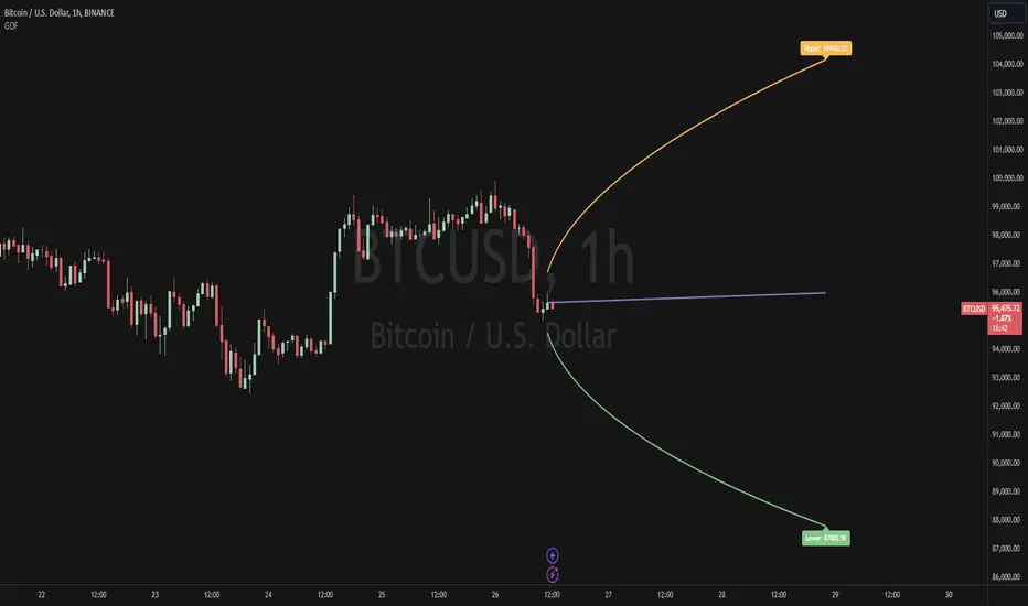
The Indicator combines volatility and frequency distributions to forecast an area of possible price expansion with an approximate confidence interval / level and level of significance (significance level).

The Script Formula



Additional comments

To alter the models forecasting precision to reflect a given confidence interval, e.g the 90% confidence level (C.L.), use the 1.64 multiplier (toggle value in "Standard normal distribution sd" setting), to use a specific C.L., e.g. the 85th percentile either search for this on google, or calculate it yourself using a Standard Normal Distribution Probability table. Additionaly volatility may be changed by toggling the lookback period setting, this can be thought of as widening the distribution tails.

The look forward parameter is currently fixed at 20, this is because it does not currently work correctly with higher integers, I will try resolve this problem and any other bugs as soon as possible

2024年12月26日

發行說明

- Fixed forecast limit to chart maximum = 100 bars of x unit time in future. Script now uses

polyline

variables to fill arrays containing

chart.point

objects data which are then plotted using instances of the polyline type ~ class)
- Price labels for chart maximum and chart minimum forecasts
- Different Forecasting types (Price, Normal, Log-Normal (this is the exponential of the normal distribution)



Model Assumptions:

For “Price”

• Normal distribution of residuals (difference between source and moving average at time i where moving average is constant)
  
• Independence of residuals (i.e. we assume residuals are iid)
  
• Stationarity of time series (we assume that the mean = moving average and variance is remains constant over the forecast horizon)
  

For “Normal” and “Log-Normal” forecasting type

• Log-Normal distribution of residuals (difference between log returns and mean sample log returns at time i where sample mean is constant over lookback period)
  
• Independence of residuals (i.e. we assume residuals are iid)
  
• Stationarity of drift (mu) and log returns (sigma)
  

Comments on the Log-Normal Forecast Model

Simulating asset-prices assuming a log-normal distribution is preferred as it models real life scenarios most accurately, e.g. it caters to the fact of non-negative prices, positive skewness and multiplicativity, assumptions that the other models fail to make.

If we were to simulate asset prices via GBM (geometric brownian motion) using the same mean and variance parameters as in our residual standard deviation and simulate n paths, we would expect the price to remain within the confidence interval (by assumption) approximately C.I amount of the time where C.I. is the confidence level corresponding to the Z score used in the residual standard deviation of log returns(e.g. a 90% C.I. means 90% of all sampled values will be less than or as extreme as the corresponding Z score value, in this case 1.64). In other words only (1 - C.I.)% of the time would we expect a more extreme prediction. This is because GBM assumes normally distributed log returns, constant drift and volatility.

Let's take the following example, we have a 95% C.I., so we expect only 5% of simulated GBM paths to lie outside our confidence interval. We can see this in action below. note by law of large numbers, the limit as n (number of simulated paths) tends to infinity of the probability that the number of values that lie within the confidence interval will tend towards its theoretical maximum identical to our C.I.