Zone Tap Counter: Support & Resistance StrengthWhat is this indicator?
This script is designed to help traders objectively monitor the strength and significance of price zones by counting and visualizing how many times price “taps” confirmed support and resistance levels. The indicator leverages swing high/low detection to automatically plot relevant zones and uses price tap frequency as an objective strength metric.
How does it work?
Zone Identification:
The script uses the Pine Script functions ta.pivothigh and ta.pivotlow to detect confirmed swing highs and lows on your chart. Each swing high establishes a resistance zone, and each swing low establishes a support zone.
Only confirmed pivots are used, ensuring all signals are strictly non-repainting.
Tap Counting Logic:
For every candle, the indicator checks whether price touches (comes within a small, user-set tolerance) of any currently tracked support or resistance zone. To avoid counting repeated taps in the same move, the script ensures only unique bar taps are registered.
Each time price taps a zone, a counter for that zone is incremented.
Both the tolerance for taps (percentage-based), and the depth/history of zones tracked are fully adjustable in settings.
Visual Feedback:
Zones with more taps are drawn darker (lower transparency), making it easy to spot the strongest/hardest-tested levels on the chart.
A label on each zone displays the current tap count (e.g., "3x"), giving direct feedback about which support/resistance are most significant in the current view.
Only recent zones (user-configurable) are shown to keep charts clear and useful.
How to use it:
Add the indicator to your TradingView chart.
Set the swing length and tap tolerance in settings to match your market or timeframe (short swing length for scalping, longer swings for bigger structure).
Watch for zones with high tap counts and darker lines: These zones represent areas where price has repeatedly reacted, suggesting they may be important for your trading decisions.
You can adjust the minimum number of taps needed for a zone to be highlighted and the number of zones to display for your preferred visual clarity.
Combine this tool with other analysis for confirmation—tap counts should not be seen as trading signals, but as supporting information.
Originality & Calculation Details:
This script does NOT simply merge or overlay existing indicators. The calculation method is original: it uses swing-based support/resistance and applies unique tap-count logic, designed for objective zone strength visualization.
No repainting logic is present.
All code and visualization methods are documented and transparent.
Disclaimer:
This indicator is for educational and analytical purposes only. It does not predict future price movement, guarantee profits, or recommend specific trades. Always use your own analysis and risk management. See TradingView’s House Rules for more details.
在腳本中搜尋"zone"

Zone Levels (Range + ZoneHeight)This is a Template for drawing out zones from one ankerpoint zone.Just mark out the distance from one leveledge to the next and it will give you infinte more zoneedges in the same distance. You can also adjust the zone height if wanted (i used 10 as example).
I hope youll enjoy it
AJ

Zone TP SL [By Gone]It creates a price zone for TP 3 Level, increasing from the price by 500 points and setting an SL zone of 500 points of the price.
You must enter the price range yourself, recommended to be 500 points apart.
1. select Type Bay And Sell
2. Input Price Start And End
suitable for gold
Made to help with hitting the price zone. For use in making decisions about trading.


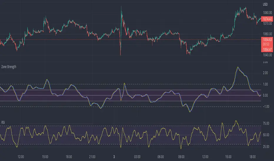
Zone Strength [wbburgin]The Zone Strength indicator is a multifaceted indicator combining volatility-based, momentum-based, and support-based metrics to indicate where a trend reversal is likely.
I recommend using it with the RSI at normal settings to confirm entrances and exits.
The indicator first uses a candle’s wick in relation to its body, depending on whether it closes green or red, to determine ranges of volatility.
The maxima of these volatility statistics are registered across a specific period (the “amplitude”) to determine regions of current support.
The “wavelength” of this statistic is taken to smooth out the Zone Strength’s final statistic.
Finally, the ratio of the difference between the support and the resistance levels is taken in relation to the candle to determine how close the candle is to the “Buy Zone” (<-0.5) or the “Sell Zone” (>0.5).
wbburgin
Zone at Period timeMark a zone every day at given period of time.
Has 4 time inputs:
- fromHour: start time of the period.
-fromMinute: minute of start of period
- toHour: period end time
-toMinute: final minute of the period
With "weekdaysOnly" it is determined if weekends are ignored.


Trend Fib Zone Bounce (TFZB) [KedArc Quant]Description:
Trend Fib Zone Bounce (TFZB) trades with the latest confirmed Supply/Demand zone using a single, configurable Fib pullback (0.3/0.5/0.6). Trade only in the direction of the most recent zone and use a single, configurable fib level for pullback entries.
• Detects market structure via confirmed swing highs/lows using a rolling window.
• Draws Supply/Demand zones (bearish/bullish rectangles) from the latest MSS (CHOCH or BOS) event.
• Computes intra zone Fib guide rails and keeps them extended in real time.
• Triggers BUY only inside bullish zones and SELL only inside bearish zones when price touches the selected fib and closes back beyond it (bounce confirmation).
• Optional labels print BULL/BEAR + fib next to the triangle markers.
What it does
Finds structure using confirmed swing highs/lows (you choose the confirmation length).
Builds the latest zone (bullish = demand, bearish = supply) after a CHOCH/BOS event.
Draws intra-zone “guide rails” (Fib lines) and extends them live.
Signals only with the trend of that zone:
BUY inside a bullish zone when price tags the selected Fib and closes back above it.
SELL inside a bearish zone when price tags the selected Fib and closes back below it.
Optional labels print BULL/BEAR + Fib next to triangles for quick context
Why this is different
Most “zone + fib + signal” tools bolt together several indicators, or fire counter-trend signals because they don’t fully respect structure. TFZB is intentionally minimal:
Single bias source: the latest confirmed zone defines direction; nothing else overrides it.
Single entry rule: one Fib bounce (0.3/0.5/0.6 selectable) inside that zone—no counter-trend trades by design.
Clean visuals: you can show only the most recent zone, clamp overlap, and keep just the rails that matter.
Deterministic & transparent: every plot/label comes from the code you see—no external series or hidden smoothing
How it helps traders
Cuts decision noise: you always know the bias and the only entry that matters right now.
Forces discipline: if price isn’t inside the active zone, you don’t trade.
Adapts to volatility: pick 0.3 in strong trends, 0.5 as the default, 0.6 in chop.
Non-repainting zones: swings are confirmed after Structure Length bars, then used to build zones that extend forward (they don’t “teleport” later)
How it works (details)
*Structure confirmation
A swing high/low is only confirmed after Structure Length bars have elapsed; the dot is plotted back on the original bar using offset. Expect a confirmation delay of about Structure Length × timeframe.
*Zone creation
After a CHOCH/BOS (momentum shift / break of prior swing), TFZB draws the new Supply/Demand zone from the swing anchors and sets it active.
*Fib guide rails
Inside the active zone TFZB projects up to five Fib lines (defaults: 0.3 / 0.5 / 0.7) and extends them as time passes.
*Entry logic (with-trend only)
BUY: bar’s low ≤ fib and close > fib inside a bullish zone.
SELL: bar’s high ≥ fib and close < fib inside a bearish zone.
*Optionally restrict to one signal per zone to avoid over-trading.
(Optional) Aggressive confirm-bar entry
When do the swing dots print?
* The code confirms a swing only after `structureLen` bars have elapsed since that candidate high/low.
* On a 5-min chart with `structureLen = 10`, that’s about 50 minutes later.
* When the swing confirms, the script plots the dot back on the original bar (via `offset = -structureLen`). So you *see* the dot on the old bar, but it only appears on the chart once the confirming bar arrives.
> Practical takeaway: expect swing markers to appear roughly `structureLen × timeframe` later. Zones and signals are built from those confirmed swings.
Best timeframe for this Indicator
Use the timeframe that matches your holding period and the noise level of the instrument:
* Intraday :
* 5m or 15m are the sweet spots.
* Suggested `structureLen`:
* 5m: 10–14 (confirmation delay \~50–70 min)
* 15m: 8–10 (confirmation delay \~2–2.5 hours)
* Keep Entry Fib at 0.5 to start; try 0.3 in strong trends, 0.6 in chop.
* Tip: avoid the first 10–15 minutes after the open; let the initial volatility set the early structure.
* Swing/overnight:
* 1h or 4h.
* `structureLen`:
* 1h: 6–10 (6–10 hours confirmation)
* 4h: 5–8 (20–32 hours confirmation)
* 1m scalping: not recommended here—the confirmation lag relative to the noise makes zones less reliable.
Inputs (all groups)
Structure
• Show Swing Points (structureTog)
o Plots small dots on the bar where a swing point is confirmed (offset back by Structure Length).
• Structure Length (structureLen)
o Lookback used to confirm swing highs/lows and determine local structure. Higher = fewer, stronger swings; lower = more reactive.
Zones
• Show Last (zoneDispNum)
o Maximum number of zones kept on the chart when Display All Zones is off.
• Display All Zones (dispAll)
o If on, ignores Show Last and keeps all zones/levels.
• Zone Display (zoneFilter): Bullish Only / Bearish Only / Both
o Filters which zone types are drawn and eligible for signals.
• Clean Up Level Overlap (noOverlap)
o Prevents fib lines from overlapping when a new zone starts near the previous one (clamps line start/end times for readability).
Fib Levels
Each row controls whether a fib is drawn and how it looks:
• Toggle (f1Tog…f5Tog): Show/hide a given fib line.
• Level (f1Lvl…f5Lvl): Numeric ratio in . Defaults active: 0.3, 0.5, 0.7 (0 and 1 off by default).
• Line Style (f1Style…f5Style): Solid / Dashed / Dotted.
• Bull/Bear Colors (f#BullColor, f#BearColor): Per-fib color in bullish vs bearish zones.
Style
• Structure Color: Dot color for confirmed swing points.
• Bullish Zone Color / Bearish Zone Color: Rectangle fills (transparent by default).
Signals
• Entry Fib for Signals (entryFibSel): Choose 0.3, 0.5 (default), or 0.6 as the trigger line.
• Show Buy/Sell Signals (showSignals): Toggles triangle markers on/off.
• One Signal Per Zone (oneSignalPerZone): If on, suppresses additional entries within the same zone after the first trigger.
• Show Signal Text Labels (Bull/Bear + Fib) (showSignalLabels): Adds a small label next to each triangle showing zone bias and the fib used (e.g., BULL 0.5 or BEAR 0.3).
How TFZB decides signals
With trend only:
• BUY
1. Latest active zone is bullish.
2. Current bar’s close is inside the zone (between top and bottom).
3. The bar’s low ≤ selected fib and it closes > selected fib (bounce).
• SELL
1. Latest active zone is bearish.
2. Current bar’s close is inside the zone.
3. The bar’s high ≥ selected fib and it closes < selected fib.
Markers & labels
• BUY: triangle up below the bar; optional label “BULL 0.x” above it.
• SELL: triangle down above the bar; optional label “BEAR 0.x” below it.
Right-Panel Swing Log (Table)
What it is
A compact, auto-updating log of the most recent Swing High/Low events, printed in the top-right of the chart.
It helps you see when a pivot formed, when it was confirmed, and at what price—so you know the earliest bar a zone-based signal could have appeared.
Columns
Type – Swing High or Swing Low.
Date – Calendar date of the swing bar (follows the chart’s timezone).
Swing @ – Time of the original swing bar (where the dot is drawn).
Confirm @ – Time of the bar that confirmed that swing (≈ Structure Length × timeframe after the swing). This is also the earliest moment a new zone/entry can be considered.
Price – The swing price (high for SH, low for SL).
Why it’s useful
Clarity on repaint/confirmation: shows the natural delay between a swing forming and being usable—no guessing.
Planning & journaling: quick reference of today’s pivots and prices for notes/backtesting.
Scanning intraday: glance to see if you already have a confirmed zone (and therefore valid fib-bounce entries), or if you’re still waiting.
Context for signals: if a fib-bounce triangle appears before the time listed in Confirm @, it’s not a valid trade (you were too early).
Settings (Inputs → Logging)
Log swing times / Show table – turn the table on/off.
Rows to keep – how many recent entries to display.
Show labels on swing bar – optional tags on the chart (“Swing High 11:45”, “Confirm SH 14:15”) that match the table.
Recommended defaults
• Structure Length: 10–20 for intraday; 20–40 for swing.
• Entry Fib for Signals: 0.5 to start; try 0.3 in stronger trends and 0.6 in choppier markets.
• One Signal Per Zone: ON (prevents over trading).
• Zone Display: Both.
• Fib Lines: Keep 0.3/0.5/0.7 on; turn on 0 and 1 only if you need anchors.
Alerts
Two alert conditions are available:
• BUY signal – fires when a with trend bullish bounce at the selected fib occurs inside a bullish zone.
• SELL signal – fires when a with trend bearish bounce at the selected fib occurs inside a bearish zone.
Create alerts from the chart’s Alerts panel and select the desired condition. Use Once Per Bar Close to avoid intrabar flicker.
Notes & tips
• Swing dots are confirmed only after Structure Length bars, so they plot back in time; zones built from these confirmed swings do not repaint (though they extend as new bars form).
• If you don’t see a BUY where you expect one, check: (1) Is the active zone bullish? (2) Did the candle’s low actually pierce the selected fib and close above it? (3) Is One Signal Per Zone suppressing a second entry?
• You can hide visual clutter by reducing Show Last to 1–3 while keeping Display All Zones off.
Glossary
• CHOCH (Change of Character): A shift where price breaks beyond the last opposite swing while local momentum flips.
• BOS (Break of Structure): A cleaner break beyond the prior swing level in the current momentum direction.
• MSS: Either CHOCH or BOS – any event that spawns a new zone.
Extension ideas (optional)
• Add fib extensions (1.272 / 1.618) for target lines.
• Zone quality score using ATR normalization to filter weak impulses.
• HTF filter to only accept zones aligned with a higher timeframe trend.
⚠️ Disclaimer This script is provided for educational purposes only.
Past performance does not guarantee future results.
Trading involves risk, and users should exercise caution and use proper risk management when applying this strategy.

EMA with Supply and Demand Zones
The EMA with Supply and Demand Strategy is a trend-following trading approach that integrates Exponential Moving Averages (EMA) with supply and demand zones to identify potential entry and exit points. Below is a detailed description of its components and logic:
Key Components of the Strategy
1. EMA (Exponential Moving Average)
The EMA is used as a trend filter:
Bullish Trend: Price is above the EMA.
Bearish Trend: Price is below the EMA.
The EMA ensures that trades align with the overall market trend, reducing counter-trend risks.
2. Supply and Demand Zones
Demand Zone:
Represents areas where the price historically found support (buyers dominated).
Calculated using the lowest low over a specified lookback period.
Used for identifying potential long entry points.
Supply Zone:
Represents areas where the price historically faced resistance (sellers dominated).
Calculated using the highest high over a specified lookback period.
Used for identifying potential short entry points.
3. Trade Conditions
Long Trade:
Triggered when:
The price is above the EMA (bullish trend).
The low of the current candle touches or penetrates the most recent demand zone.
Short Trade:
Triggered when:
The price is below the EMA (bearish trend).
The high of the current candle touches or penetrates the most recent supply zone.
4. Exit Conditions
Long Exit:
Exit the trade when the price closes below the EMA, indicating a potential trend reversal.
Short Exit:
Exit the trade when the price closes above the EMA, signaling a potential upward reversal.
Visual Representation
EMA: A blue line plotted on the chart to show the trend.
Supply Zones: Red horizontal lines representing potential resistance levels.
Demand Zones: Green horizontal lines representing potential support levels.
These zones dynamically adjust to reflect the most recent 3 levels.
How the Strategy Works
Trend Identification:
The EMA determines the direction of the trade:
Look for long trades only in a bullish trend (price above EMA).
Look for short trades only in a bearish trend (price below EMA).
Entry Points:
Wait for price interaction with a supply or demand zone:
If the price touches a demand zone during a bullish trend, initiate a long trade.
If the price touches a supply zone during a bearish trend, initiate a short trade.
Risk Management:
The strategy exits trades if the price moves against the trend (crosses the EMA).
This ensures minimal exposure during adverse market movements.
Benefits of the Strategy
Trend Alignment:
Reduces counter-trend trades, improving the win rate.
Clear Entry and Exit Rules:
Combines price action (zones) with a reliable trend filter (EMA).
Dynamic Levels:
The supply and demand zones adapt to changing market conditions.
Customization Options
EMA Length:
Adjust to suit different timeframes or market conditions (e.g., 20 for faster trends, 50 for slower trends).
Lookback Period:
Fine-tune to capture broader or narrower supply and demand zones.
Risk/Reward Preferences:
Pair the strategy with stop-loss and take-profit levels for enhanced control.
This strategy is ideal for traders looking for a structured approach to identify high-probability trades while aligning with the prevailing trend. Backtest and optimize parameters based on your trading style and the specific asset you're tradin

Momentum Shift [Bigbeluga]
This indicator identifies momentum shifts using a smoothed momentum calculation. It plots dynamic shift zones consisting of five levels that expand or contract based on price action. When momentum rises, the indicator creates an upward shift zone, and when momentum falls, it generates a downward shift zone. The shift zones dynamically react to price, stopping extension when a level is crossed.
🔵Key Features:
Smoothed Momentum Calculation:
➣ Utilizes a Hull Moving Average (HMA) to smooth momentum and reduce noise.
➣ Identifies momentum shifts with crossovers between the current momentum value and its previous state.
➣ Uses a gradient color scheme to highlight momentum strength.
Dynamic Shift Zones:
➣ When momentum rises, the indicator plots an upper shift zone with five incremental levels.
➣ When momentum falls, a lower shift zone is formed with five descending levels.
➣ Each level within the shift zone represents a progressively stronger momentum shift.
Level Extension Control:
➣ Shift zones stop extending once a level is crossed by price.
➣ Levels closer to price act as key momentum resistance or support zones.
➣ If price retraces after a shift, the remaining levels stay intact for further reference.
Momentum Direction Indications:
➣ Labels (▲ and ▼) appear at momentum shift points to indicate rising or falling momentum.
🔵Usage:
Momentum-Based Entries: Identify momentum shifts early by using shift zones as confirmation for trade entries.
Trend Continuation & Exhaustion: Observe which shift levels price respects—if momentum shift zones hold, the trend may continue; if they break, momentum may reverse.
Dynamic Support & Resistance: Use the five-level shift zones as temporary support and resistance areas that adapt to momentum shifts.
Momentum Strength Analysis: If price moves through multiple shift levels in one direction, it signals strong momentum in that direction.
Momentum Shift is a powerful tool for traders looking to analyze momentum shifts with structured visual zones. By combining smoothed momentum calculations with dynamic shift zones, this indicator provides a clear view of market momentum and helps traders navigate price action effectively.

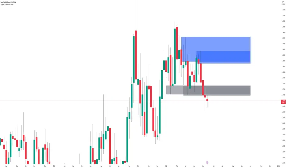
Support and Resistance ZonesSupport and Resistance Zones— Indicator
Overview :
This indicator dynamically detects and visualizes key support and resistance zones by aggregating price data into synthetic candles. It highlights these critical price areas as shaded boxes that adjust in real-time, providing traders with clear visual cues on where price might find support or resistance.
Key Features :
-Dynamic Zone Detection: Automatically identifies zones formed by consecutive grouped candles meeting customizable criteria.
-Aggregation Factor: Combine multiple bars into synthetic candles to reduce noise and emphasize significant price zones.
-Customizable Zone Length: Extend the zone boxes by a user-defined number of bars beyond the current price for enhanced visualization.
-Visual Styling: Fully customizable zone fill and border colors to suit your chart preferences.
-Zone Lifecycle Control: Option to terminate old zones to maintain a clean chart.
-Breakout Alerts: Trigger alerts when price breaks above or below confirmed zones, signaling potential trading opportunities.
Inputs :
-Minimum Candles to Form Zone: Sets how many consecutive synthetic candles must align to form a valid zone.
-Aggregation Factor: Defines how many bars are combined to create a synthetic candle.
-Zone Fill and Border Colors: Customize the appearance of zones on the chart.
-Terminate Old Zones: Enable or disable automatic removal of previous zones.
-Box Extension Bars: Number of bars the zone boxes extend beyond their detected range for better visibility.
How to Use :
1. Apply the Indicator : Add it to your chart on any timeframe or market (Forex, stocks, crypto).
2. Set Input : Adjust the minimum candles, aggregation factor, and box extension bars based on your trading style and timeframe. For example, higher aggregation smooths noise for longer-term zones.
3. Visualize Zones : Watch as the indicator dynamically draws shaded boxes representing areas of support and resistance. Zones will grow as price action confirms their strength.
4. Monitor Breakouts : Use breakout alerts to be notified when price decisively moves beyond a zone, providing signals for possible entries or exits.
5.Customize Appearance : Adjust colors and enable zone termination to keep your chart clear and focused.
This tool simplifies identifying important price levels, reducing manual analysis time and helping you make informed trading decisions.

Dynamic Supply & Demand Zones- AYNETSummary of the Code: Dynamic Supply & Demand Zones
This Pine Script creates dynamic supply (resistance) and demand (support) zones on a chart by identifying the highest and lowest prices over a user-defined lookback period. It visualizes these zones with shaded regions and horizontal lines that dynamically adjust to price movements.
Key Features:
Dynamic Support Zone (Demand):
Calculated using the lowest price in the last lookback bars.
Creates a shaded region around this price, extended up and down by a user-defined zone width.
Horizontal lines clearly mark the top and bottom of the demand zone.
Dynamic Resistance Zone (Supply):
Calculated using the highest price in the last lookback bars.
Similarly, a shaded region and lines are drawn for this zone, representing supply.
Customizable Inputs:
lookback: Number of bars to calculate the highest and lowest prices.
zone_width: The buffer distance above/below the highest/lowest price to create the zone.
Colors: Separate color inputs for the fill and lines of support and resistance zones.
Dynamic Updates:
Both zones update automatically as new bars are added and the highest/lowest prices change.
Visual Representation:
The script uses plot to create shaded regions and line objects to draw horizontal boundaries.
How It Works:
Inputs:
The user provides a lookback period and zone_width.
Calculations:
Lowest price in the last lookback bars defines the support zone.
Highest price in the same period defines the resistance zone.
Plotting:
The zones are plotted with shaded regions and dynamic lines.
Use Case:
This indicator helps identify key price levels where supply (resistance) or demand (support) is likely to affect price movement.
Useful for traders who rely on support/resistance levels in their strategies.
Let me know if you'd like further enhancements or integrations! 😊

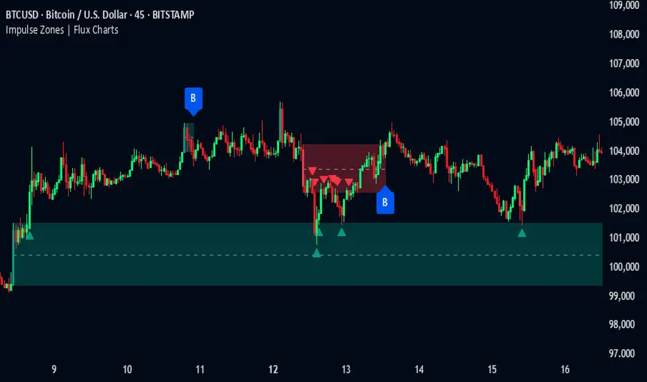
Impulse Zones | Flux Charts💎 GENERAL OVERVIEW
Introducing our new Impulse Zones indicator, a powerful tool designed to identify significant price movements accompanied by strong volume, highlighting potential areas of support and resistance. These Impulse Zones can offer valuable insights into market momentum and potential reversal or continuation points. For more information about the process, please check the "HOW DOES IT WORK ?" section.
Impulse Zones Features :
Dynamic Zone Creation : Automatically identifies and plots potential supply and demand zones based on significant price impulses and volume spikes.
Customizable Settings : Allows you to adjust the sensitivity of zone detection based on your trading style and market conditions.
Retests and Breakouts : Clearly marks instances where price retests or breaks through established Impulse Zones, providing potential entry or exit signals.
Alerts : You can set alerts for Bullish & Bearish Impulse Zone detection and their retests.
🚩 UNIQUENESS
Our Impulse Zones indicator stands out by combining both price action (impulsive moves) and volume confirmation to define significant zones. Unlike simple support and resistance indicators, it emphasizes the strength behind price movements, potentially filtering out less significant levels. The inclusion of retest and breakout visuals directly on the chart provides immediate context for potential trading opportunities. The user can also set up alerts for freshly detected Impulse Zones & the retests of them.
📌 HOW DOES IT WORK ?
The indicator identifies bars where the price range (high - low) is significantly larger than the average true range (ATR), indicating a strong price movement. The Size Sensitivity input allows you to control how large this impulse needs to be relative to the ATR.
Simultaneously, it checks if the volume on the impulse bar is significantly higher than the average volume. The Volume Sensitivity input governs this threshold.
When both the price impulse and volume confirmation criteria are met, an Impulse Zone is created in the corresponding direction. The high and low of the impulse bar define the initial boundaries of the zone. Zones are extended forward in time to remain relevant. The indicator manages the number of active zones to maintain chart clarity and can remove zones that haven't been touched for a specified period. The indicator monitors price action within and around established zones.
A retest is identified when the price touches a zone and then moves away. A break occurs when the price closes beyond the invalidation point of a zone. Keep in mind that if "Show Historic Zones" setting is disabled, you will not see break labels as their zones will be removed from the chart.
The detection of Impulse Zones are immediate signs of significant buying or selling pressure entering the market. These zones represent areas where a strong imbalance between buyers and sellers has led to a rapid price movement accompanied by high volume. Bullish Impulse Zones act as a possible future support zone, and Bearish Impulse Zones act as a possible future resistance zone. Retests of the zones suggest a strong potential movement in the corresponding direction.
⚙️ SETTINGS
1. General Configuration
Show Historic Zones: If enabled, invalidated or expired Impulse Zones will remain visible on the chart.
2. Impulse Zones
Invalidation Method: Determines which part of the candle (Wick or Close) is used to invalidate a zone break.
Size Sensitivity: Controls the required size of the impulse bar relative to the ATR for a zone to be detected. Higher values may identify fewer, larger zones. Lower values may detect more, smaller zones.
Volume Sensitivity: Controls the required volume of the impulse bar relative to the average volume for a zone to be detected. Higher values require more significant volume.
Labels: Toggles the display of "IZ" labels on the identified zones.
Retests: Enables the visual highlighting of retests on the zones.
Breaks: Enables the visual highlighting of zone breaks.
Machine Learning-Inspired Supply & Demand Zones [AlgoPoint]This indicator is a Smart Supply & Demand Zone tool, developed with principles inspired by Machine Learning (ML). It intelligently filters out market noise, allowing you to focus only on the most significant zones where institutional order flow is likely present.
💡 How It Works: Why Is This Indicator "Smart"?
Unlike traditional indicators that only measure simple price movements, this script uses an algorithm that asks the same critical questions an experienced market analyst would to qualify a zone:
- 1. Price Imbalance: How fast and aggressively did the price leave the zone? Our algorithm measures the body size of the "departure candle" relative to the current market volatility (ATR). A zone is only considered if it was formed by an explosive move that is statistically significant, indicating a major imbalance between buyers and sellers.
- 2. Volume Confirmation: Did the "smart money" participate in this move? The script checks if the volume on the departure candle was significantly higher than the recent average volume. A spike in volume confirms that the move was backed by institutional interest, adding strength and validity to the zone.
- 3. Valid Pivot Structure: Did the zone originate from a meaningful swing high or low? The algorithm first identifies a valid pivot structure, ensuring that zones are not drawn from insignificant or random price fluctuations.
Only when a potential zone passes these three critical tests—our "quality filter"—is it drawn on your chart.
🚀 Features & How to Use
Using the indicator is straightforward. You will see two primary types of boxes on your chart:
* 🟥 Red Box (Supply Zone): An area of potential resistance where selling pressure is likely to be strong. Look for potential shorting opportunities as the price approaches this zone.
* 🟩 Green Box (Demand Zone): An area of potential support where buying pressure is likely to be strong. Look for potential long opportunities as the price pulls back into this zone.
Dynamic Zone Management
This indicator is not static; it lives and breathes with the market:
- Fresh Zone: A newly formed zone appears in its full, vibrant color. These are the highest-probability zones as they have not yet been re-tested.
- Broken / Flipped Zone: You have full control over what happens when a zone is broken! In the settings, you can choose:
- Delete Zone: The zone will be removed completely when the price closes through it.
- Show as Broken (Flip): When broken, the zone will turn gray, stop extending, and remain on your chart. This is extremely useful for identifying Support/Resistance Flips, where a broken demand zone becomes new resistance, or a broken supply zone becomes new support.
⚙️ Settings & Customization
Fine-tune the indicator to match your personal trading style via the settings menu:
- Breakout Behavior: The most powerful feature. Choose between Delete Zone and Show as Broken (Flip) to customize your chart.
- Zone Finding Logic: Control the indicator's sensitivity.
- Selective: Requires both strong imbalance and high volume. Finds fewer, but higher-quality, zones.
- Moderate: Requires either strong imbalance or high volume. Finds more potential zones.
- Sensitivity Settings: Adjust the ATR Multiplier and Volume Multiplier to make the criteria for a "strong" zone stricter or looser.
Frozen Bias Zones – Sentiment Lock-insOverview
The Frozen Bias Zones indicator visualizes market sentiment lock-ins using a combination of RSI, MACD, and OBV. It creates "bias zones" that indicate whether the market is in a sustained bullish or bearish phase. These zones are then highlighted on the chart, helping traders spot when the market is locked in a bias. The script also detects breakout events from these zones and marks them with clear labels for easier decision-making.
Features
Multi-Indicator Sentiment Analysis: Combines RSI, MACD, and OBV to detect synchronized bullish or bearish sentiment.
Frozen Bias Zones: Identifies and visually represents zones where the market has remained in a particular sentiment (bullish or bearish) for a defined period.
Breakout Alerts: Displays labels to indicate when the price breaks out of the established bias zone.
Customizable Inputs: Adjust the zone duration, RSI, MACD, and breakout label visibility.
Input Parameters
Bias Duration (biasLength)
The minimum number of candles the market must stay in a specific sentiment to consider it a "Frozen Bias Zone".
Default: 5 candles.
RSI Period (rsiPeriod)
Period for the Relative Strength Index (RSI) calculation.
Default: 14 periods.
MACD Settings
MACD Fast (macdFast): The fast-moving average period for the MACD calculation.
Default: 12.
MACD Slow (macdSlow): The slow-moving average period for the MACD calculation.
Default: 26.
MACD Signal (macdSig): The signal line period for MACD.
Default: 9.
Show Break Label (showBreakLabel)
Toggle to show labels when the price breaks out of the bias zone.
Default: True (shows label).
Bias Zone Colors
Bullish Bias Color (bullColor): The color for bullish zones (light green).
Bearish Bias Color (bearColor): The color for bearish zones (light red).
How It Works
This indicator analyzes three key market metrics to determine whether the market is in a bullish or bearish phase:
RSI (Relative Strength Index)
Measures the speed and change of price movements. RSI > 50 indicates a bullish phase, while RSI < 50 indicates a bearish phase.
MACD (Moving Average Convergence Divergence)
Measures the relationship between two moving averages of the price. A positive MACD histogram indicates bullish momentum, while a negative histogram indicates bearish momentum.
OBV (On-Balance Volume)
Uses volume flow to determine if a trend is likely to continue. A rising OBV indicates bullish accumulation, while a falling OBV indicates bearish distribution.
Bias Zone Detection
The market sentiment is considered bullish if all three indicators (RSI, MACD, and OBV) are bullish, and bearish if all three indicators are bearish.
Bullish Zone: A zone is created when the market sentiment remains bullish for the duration of the specified biasLength.
Bearish Zone: A zone is created when the market sentiment remains bearish for the duration of the specified biasLength.
These bias zones are visually represented on the chart as colored boxes (green for bullish, red for bearish).
Breakout Detection
The script automatically detects when the market exits a bias zone. If the price moves outside the bounds of the established zone (either up or down), the script will display one of the following labels:
Bias Break (Up): Indicates that the price has broken upwards out of the zone (with a green label).
Bias Break (Down): Indicates that the price has broken downwards out of the zone (with a red label).
These labels help traders easily identify potential breakout points.
Example Use Case
Bullish Market Conditions: If the RSI is above 50, the MACD histogram is positive, and OBV is increasing, the script will highlight a green bias zone. Traders can watch for potential bullish breakouts or trend continuation after the zone ends.
Bearish Market Conditions: If the RSI is below 50, the MACD histogram is negative, and OBV is decreasing, the script will highlight a red bias zone. Traders can look for potential bearish breakouts when the zone ends.
Conclusion
The Frozen Bias Zones indicator is a powerful tool for traders looking to visualize prolonged market sentiment, whether bullish or bearish. By combining RSI, MACD, and OBV, it helps traders spot when the market is "locked in" to a bias. The breakout labels make it easier to take action when the price moves outside of the established zone, potentially signaling the start of a new trend.
Instructions
To use this script:
Add the Frozen Bias Zones indicator to your TradingView chart.
Adjust the input parameters to suit your trading strategy.
Observe the colored bias zones on your chart, along with breakout labels, to make informed decisions on trend continuation or reversal.

Support & Resistance ZonesTitle: A Comprehensive Guide to the Support & Resistance Zones Indicator
Introduction
In the world of technical analysis, the Support & Resistance Zones indicator plays a crucial role in identifying potential trading opportunities. These zones are essential for traders looking to capitalize on bounces or break and retests. In this article, we will delve into the specifics of the Support & Resistance Zones indicator, outlining how it works, how it finds and marks zones, and the various options available for traders.
What the indicator is about
The Support & Resistance Zones indicator, developed by @HarryCTC, is a powerful tool for detecting areas of potential price reversal or consolidation in a financial market. These zones are significant as they can act as a guide for traders to make informed decisions on entering or exiting positions. Specifically, the indicator helps identify:
1. Support Zones: Areas where the price has a tendency to bounce back up after falling, indicating a potential buying opportunity.
2. Resistance Zones: Areas where the price has a tendency to reverse after rising, indicating a potential selling opportunity.
How the indicator finds its zones
The Support & Resistance Zones indicator utilizes pivot points to identify potential support and resistance levels. By analyzing the fractal structure of the price chart, the indicator identifies key turning points, known as bull and bear fractals. The bull fractal is a high pivot point, while the bear fractal is a low pivot point.
The fractal structure is determined by the 'Switch Zone Period' input, which can be adjusted to suit the trader's preferences. A higher value will result in fewer zones being identified, while a lower value will result in more zones.
How it marks zones and why it marks zones
The indicator marks the support and resistance zones by creating rectangular boxes around the identified fractal points. The zones are extended horizontally from the fractal point, allowing traders to visualize the potential areas of price reversal.
The zones are marked for the following reasons:
1. To provide a clear visual representation of potential support and resistance levels.
2. To help traders identify potential entry and exit points based on the price's reaction to these zones.
3. To serve as a reference for stop-loss and take-profit levels when planning trades.
The indicator's for traders trading bounces or break and retests
Traders who focus on trading bounces or break and retests can benefit immensely from the Support & Resistance Zones indicator. By providing a visual representation of key support and resistance levels, the indicator enables traders to:
1. Identify potential buying opportunities at support zones where the price is likely to bounce back up.
2. Identify potential selling opportunities at resistance zones where the price is likely to reverse after rising.
3. Make informed decisions on stop-loss and take-profit levels based on the price's proximity to support and resistance zones.
4. Monitor the market for potential breakouts or breakdowns when the price breaches these zones.
Indicator options
The Support & Resistance Zones indicator offers several customizable options to suit the trader's preferences. These options include:
1. Switch Zone Period: Adjusts the number of periods used to calculate the fractal structure, influencing the number of identified zones.
2. No. of Displayed Zones: Determines the maximum number of zones displayed on the chart, ranging from 1 to 8.
3. Zone Extension: Adjusts the horizontal extension of the support and resistance zones.
4. Resistance Zone Color: Customizes the color of the resistance zone boxes.
5. Support Zone Color: Customizes the color of the support zone boxes.
6. Zone Border Color: Customizes the color of the zone box borders.
Conclusion
The Support & Resistance Zones indicator is a valuable tool for traders looking to identify potential trading opportunities based on the price's interaction with support and resistance levels. By providing a clear visual representation of these zones, the
indicator allows traders to make informed decisions on entry and exit points, stop-loss, and take-profit levels. With customizable options, the indicator can be tailored to suit individual trading preferences and strategies.
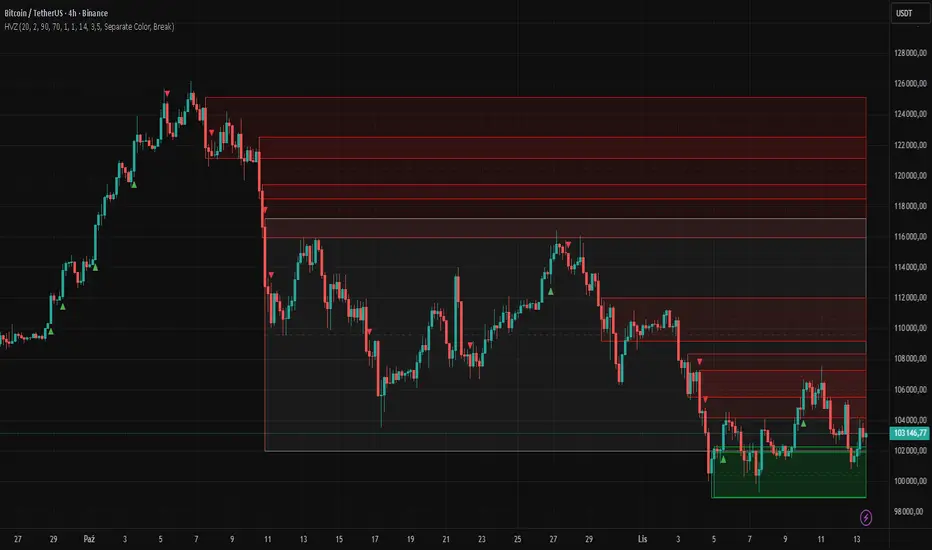
High Volume Zones with Signals – HVZ█ OVERVIEW
"High Volume Zones with Signals – HVZ" is a technical analysis indicator that identifies High Volume Zones (HVZ) on the chart and draws them as fully customizable boxes. Perfect for traders using price action, ICT, and Smart Money Concepts. The indicator highlights key volume-based support/resistance levels, detects potential consolidation zones (very large candles), and generates precise breakout and exit signals. Flexible volume filters, ATR filter, and visual styling options ensure a clean and highly effective chart.
█ CONCEPTS
The indicator detects candles with volume significantly above the average (default ≥ 2× SMA of volume over 20 periods). Such candles often signal institutional activity and create strong supply/demand zones.
The ATR filter additionally identifies very large candles – frequently a sign of market capitulation (panic buying/selling). Within the range of such a candle, prolonged consolidation often occurs, especially on higher timeframes (e.g., 4H and above).
Why are HVZ important? High-volume zones are areas where the market has left a large number of orders – institutions return there to “refresh” liquidity before the next move. A breakout against the zone’s character triggers a Break signal:
- Bullish HVZ broken downward (close below the lower boundary) → Break Down (sell),
- Bearish HVZ broken upward (close above the upper boundary) → Break Up (buy).
Note: The indicator requires real exchange volume – it will not work correctly on instruments without reported volume (e.g., certain CFDs or forex).
█ FEATURES
- HVZ Detection: Automatic identification of high-volume zones with Volume SMA Length and Volume Multiplier filters; historical initialization up to 500 candles back.
- ATR Filter: Optional detection of very large candles (potential consolidation/capitulation) using - ATR Length and ATR Multiplier; three action modes:
Skip Zone – large candle creates no zone,
Separate Color – zone is drawn in a distinct style (gray by default),
Normal Zone – treated like a regular HVZ.
- Gray zones (large candles, Separate Color): generate exactly the same Break signals as regular zones – based solely on the original candle direction (bullish → Break Down on lower break, bearish → Break Up on upper break). Gray color is only a visual marker for potential consolidation/capitulation zones.
- Customizable Boxes: Separate styles for bullish and bearish zones (border color, background gradient, line thickness and style); adjustable background and 50 % midline transparency.
- Break & Exit Signals:
Break Up/Down – green/red triangle after a candle closes outside the zone (zone disappears, triangle remains as a trace).
Exit Up/Down – green/red circle when price leaves the zone without a full breakout.
Signal Type option: Break, Exit, or Both.
- Midline: Automatic dashed line at the 50 % zone level with independent transparency control.
- Chart Cleanup: Automatic removal of inactive zones older than 500 candles (max_boxes_count=500).
- Alerts: Built-in alerts for Break Up and Break Down with clear messages.
█ HOW TO USE
Add to Chart: Paste the script in Pine Editor or find it in TradingView’s indicator library.
Configure Settings:
- Volume Filter: Volume SMA Length (default 20) and Volume Multiplier (default 2.0) – higher multiplier = fewer but stronger zones.
- ATR Filter: Enable/disable, set ATR Length (14) and ATR Multiplier (3.5); choose action for very large candles (Skip Zone / Separate Color / Normal Zone).
- Box Style: Background transparency (90) and midline transparency (70).
- Bull/Bear Box Style: Border and gradient colors, line thickness (1-5).
- ATR Style: Separate colors for large-candle zones (gray by default).
- Signal Settings: Choose Signal Type (Break/Exit/Both) and signal colors.
Signal Interpretation:
- Break Up (green triangle below bar): Bearish HVZ broken upward → buy signal, continuation of uptrend.
- Break Down (red triangle above bar): Bullish HVZ broken downward → sell signal, continuation of downtrend.
- Exit Up/Down (circles): Price leaves zone without breakout – may signal end of correction or reversal setup.
- HVZ Zones: Price often returns to high-volume zones to clear orders. An unfilled zone remains a price magnet.
- 50 % Level (midline): Ideal target for partial take-profit or reaction point inside the zone.
Combine signals with other tools (e.g., RSI, MACD, higher timeframes) for higher confidence.
█ APPLICATIONS
- Price Action & ICT: HVZ act as dynamic S/R; in an uptrend look for buys after breaking a bearish HVZ, in a downtrend look for sells after breaking a bullish HVZ. If you trade retests instead of breakouts, increase Volume Multiplier to 2.5-3.0 – fewer zones but much stronger. Note that after breaking a very strong zone, price often pulls back deeply before continuing.
- Breakout Strategies: For maximum Break signals, lower Volume Multiplier to 1.5-1.8 – gives many high-quality entries in trending markets. Always trade in the direction of the prevailing trend (e.g., only longs in uptrends). Enter after a Break signal with confirmation from volume or momentum (MACD above zero, RSI >50 for longs, <50 for shorts).
█ NOTES
- The indicator requires real exchange volume – it will not function properly on instruments without reported volume (e.g., certain CFDs, forex).
- Always confirm signals with additional context (market structure, higher timeframe).
Quantura - Supply & Demand Zone DetectionIntroduction
“Quantura – Supply & Demand Zone Detection” is an advanced indicator designed to automatically detect and visualize institutional supply and demand zones, as well as breaker blocks, directly on the chart. The tool helps traders identify key areas of market imbalance and potential reversal or continuation zones, based on price structure, volume, and ATR dynamics.
Originality & Value
This indicator provides a unique and adaptive method of zone detection that goes beyond simple pivot or candle-based logic. It merges multiple layers of confirmation—volume sensitivity, ATR filters, and swing structure—while dynamically tracking how zones evolve as the market progresses. Unlike traditional supply and demand indicators, this script also detects and plots Breaker Zones when previous imbalances are violated, giving traders an extra layer of market context.
The key values of this tool include:
Automated detection of high-probability supply and demand zones.
Integration of both volume and ATR filters for precision and adaptability.
Dynamic zone merging and updating based on price evolution.
Identification of breaker blocks (invalidated zones) to visualize market structure shifts.
Optional bullish and bearish trade signals when zones are retested.
Clear, visually optimized plotting for efficient chart interpretation.
Functionality & Core Logic
The indicator continuously scans recent price data for swing highs/lows and combines them with optional volume and ATR conditions to validate potential zones.
Demand Zones are formed when price action indicates accumulation or a strong bullish rejection from a low area.
Supply Zones are created when distribution or strong bearish rejection occurs near local highs.
Breaker Blocks appear when existing zones are invalidated by price, helping traders visualize potential market structure shifts.
Bullish and bearish signals appear when price re-enters an active zone or breaks through a breaker block.
Parameters & Customization
Demand Zones / Supply Zones: Enable or disable each individually.
Breaker Zones: Activate breaker block detection for invalidated zones.
Volume Filter: Optional filter to only confirm zones when volume exceeds its long-term average by a user-defined multiplier.
ATR Filter: Optional filter for volatility confirmation, ensuring zones form under strong momentum conditions.
Swing Length: Controls the number of bars used to detect structural pivots.
Sensitivity Controls: Adjustable ATR and volume multipliers to fine-tune detection responsiveness.
Signals: Toggle for on-chart bullish (▲) and bearish (▼) signal plotting when price interacts with zones.
Color Customization: User-defined bullish and bearish colors for both standard and breaker zones.
Core Calculations
Zones are detected using pivot highs and lows with a defined lookback and lookahead period.
Additional filters apply if ATR and volume are enabled, requiring conditions like “ATR > average * multiplier” and “Volume > average * multiplier.”
Detected zones are merged if overlapping, keeping the chart clean and logical.
When price breaks through a zone, the original box is closed, and a new breaker zone is plotted automatically.
Bullish and bearish markers appear when zones are retested from the opposite side.
Visualization & Display
Demand zones are shaded in semi-transparent bullish color (default: blue).
Supply zones are shaded in semi-transparent bearish color (default: red).
Breaker zones appear when previous imbalances are broken, helping to spot structural shifts.
Optional arrows (▲ / ▼) indicate potential buy or sell reactions on zone interaction.
Use Cases
Identify institutional areas of accumulation (demand) or distribution (supply).
Detect potential breakout traps and market structure shifts using breaker zones.
Combine with other tools such as volume profile, EMA, or liquidity indicators for deeper confirmation.
Observe retests and reactions of zones to anticipate possible reversals or continuations.
Apply multi-timeframe analysis to align higher timeframe zones with lower timeframe entries.
Limitations & Recommendations
The indicator does not predict future price movement; it highlights structural imbalances only.
Performance depends on chosen swing length and sensitivity—users should optimize parameters for each market.
Works best in volatile markets where supply and demand imbalances are clearly expressed.
Should be used as part of a broader trading framework, not as a standalone signal generator.
Markets & Timeframes
The “Quantura – Supply & Demand Zone Detection” indicator is suitable for all asset classes including cryptocurrencies, Forex, indices, commodities, and equities. It performs reliably across multiple timeframes, from intraday scalping to higher timeframe swing analysis.
Author & Access
Developed 100% by Quantura. Published as a Open-source script indicator. Access is free.
Important
This description complies with TradingView’s Script Publishing and House Rules. It clearly explains the indicator’s originality, underlying logic, functionality, and intended use without unrealistic claims or performance guarantees.

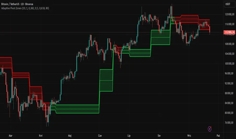
Adaptive Pivot Zones█ OVERVIEW
The "Adaptive Pivot Zones" indicator is a versatile tool designed to identify and visualize key pivot levels directly on the price chart. By detecting pivot highs and lows, the indicator calculates dynamic support and resistance zones based on user-defined levels (default: 0.382, 0.5, 0.618). These zones adapt to market volatility, providing traders with clear visual cues for potential reversal or continuation points. The indicator offers extensive customization options, such as adjusting colors, smoothing lines, and setting fill transparency, making it highly adaptable to various trading styles.
█ CONCEPTS
The "Adaptive Pivot Zones" indicator simplifies the identification of significant price levels by plotting three dynamic pivot lines, which can be smoothed to reduce market noise. The indicator dynamically changes the colors of the lines and fill zones based on price action, using bullish, bearish, or neutral colors to reflect market sentiment.
█ CALCULATIONS
The indicator relies on the following calculations:
- Pivot Detection: Pivot highs (ta.pivothigh) and pivot lows (ta.pivotlow) are identified using a user-defined pivot length (default: 10). Pivots represent significant price peaks and troughs. Higher pivot length values produce more stable levels but introduce a delay equal to the set value. For more aggressive strategies, the pivot length can be reduced.
- Pivot Levels: When both a pivot high and low are detected, the range between them is calculated (rng = drHigh - drLow). Three pivot levels are computed as:
Line 1: drLow + rng * pivotLevel1
Line 2: drLow + rng * pivotLevel2
Line 3: drLow + rng * pivotLevel3
- Smoothing: Pivot lines can be smoothed using a simple moving average (SMA) with a user-defined smoothing length (default: 1) to reduce noise and improve readability.
- Color Logic: Lines and fill zones are colored based on the price position relative to the pivot zones:
If the price is below the lowest pivot line, a bearish color is used (default: red).
If the price is above the highest pivot line, a bullish color is used (default: green).
If the price is within the pivot zones and the neutral color option is enabled, a neutral color is used (default: gray); otherwise, the previous color is retained.
- Fill Zones: The areas between pivot lines are filled with a user-defined transparency level (default: 80) to visually highlight support and resistance zones.
█ INDICATOR FEATURES
- Dynamic Pivot Lines: Three adaptive pivot lines (default levels: 0.382, 0.5, 0.618) are plotted on the price chart, adjusting to market volatility.
- Smoothing: User-defined smoothing length (default: 1) for pivot lines to reduce noise and enhance signal clarity.
- Dynamic Coloring: Lines and fill zones change color based on price action (bullish, bearish, or neutral when the price moves within the zone), reflecting market sentiment.
- Fill Zones: Transparent fills between pivot lines to visually highlight support and resistance zones.
- Customization: Options to adjust pivot length, pivot levels, smoothing, colors, transparency, and enable/disable neutral color logic.
█ HOW TO SET UP THE INDICATOR
- Add the "Adaptive Pivot Zones" indicator to your TradingView chart.
- Configure parameters in the settings, such as pivot length, pivot levels, smoothing length, and colors, to align with your trading strategy. Without smoothing, lines behave like levels; with smoothing, they act like bands. All three levels can be set to the same value to obtain a single level or a line behaving like a moving average derived from pivots.
- Enable or disable the neutral color option (for prices moving within the zone) and adjust fill transparency for optimal visualization.
- Adjust line thickness and style in the "Style" section to improve chart readability.
Example of bands – lines behave like support/resistance zones.
Example of a moving average derived from pivots – line behaves like a pivot-based MA.
█ HOW TO USE
Add the indicator to your chart, adjust the settings, and observe price interactions with the pivot lines and zones to identify potential trading opportunities. Key signals include:
- Price Interaction with Pivot Lines: When the price approaches or crosses a pivot line, it may indicate a potential support or resistance level. A bounce from a pivot line could signal a reversal, while a breakout might suggest trend continuation.
- Zone-Based Signals and Trend Line Usage: Price movement within or outside the filled zones can indicate market sentiment. Price below the lowest pivot line suggests bearish momentum, price above the highest pivot line suggests bullish momentum, and price within the zones may indicate consolidation. With higher pivot length values, the indicator can be used as a trend line, particularly during clear market movements.
- Color Changes: Shifts in line and fill colors (bullish, bearish, or neutral) provide visual cues about changing market conditions.
- Confirmation with Other Tools: Combine the indicator with tools like RSI or Bollinger Bands to validate signals and improve trade accuracy. For example, a buy signal from RSI in the oversold zone combined with a bounce from the lowest pivot line may indicate a strong entry point.
Thrax - Intraday Market Pressure ZonesTHRAX - INTRADAY MARKET PRESSURE ZONES
This indicator identifies potential support and resistance zones based on areas of significant market pressure. It dynamically plots these zones and adjusts their visibility based on real-time price action and user-defined thresholds. The indicator is useful for traders seeking to understand intraday market pressure, visualize zones of potential price reversals, and analyze volume imbalances at critical levels.
1. Support/Resistance Zones: Wherever the price retraces significantly from its high a support zone is drawn and when it retraces significantly from it low a resistance zone is drawn. The significant retracing is measured by the wick threshold percentage. For instance, if set to 75%, it implies price retracement of 75% either from high or from low for a particular candel
Volume delat: Displays volume delta information where the zones are formed. This can be used by trader to consider only those zones where delta is significant.
2. Breakout Detection: Monitors for price breakouts beyond established zones, deleting zones that are invalidated by price movement. when the price breaks a given zone with the threshold, it is considered to be mitigated and chances of trend continuation is decent.
Candle Coloring: Uses color codes (green, red, and yellow) to represent bullish, bearish, and indecisive (doji) candles, aiding quick visual assessment.
INPUTS
1. Wick Threshold (%) : Sets the minimum wick percentage required for a candle to be considered a support or resistance candidate.
2. Breakout Threshold (%) : Determines the percentage above or below a support or resistance zone that defines a breakout condition. if breaks a zone with the set threshold then the zone will be considered mititgated.
3. Max Number of Support/Resistance Zones : Limits the maximum number of support/resistance zones displayed on the chart, ranging from 1 to 5.
4. Show Wick Percentage Labels : Toggles the display of percentage values for upper and lower wicks on each candle.
TRADE SETUP
Identifying Entry Points: Look for the formation of support or resistance zones. Wait for price to retrace to these zones. if you are willing to take risk, you can consider even zones with low delta. If you want to be more cautious you should consider zones with high delta.
Volume Confirmation: Use the volume information to confirm the strength of the zone. Strong volume differences (displayed as labels) can indicate significant market pressure at these levels.
Breakout Trades: If price breaks through a support/resistance zone by more than the breakout threshold, consider this a signal for a potential trend continuation in the breakout direction.
Risk Management: Set stop-loss levels slightly outside of the identified zones to minimize risk in case of false breakouts. This can be set in input setting for breakout threshold.
Bonus Tip : Mark your significant highs and lows from where prices have retraced multiple times in the near past and if the zone is near these levels it can serve s a strong candidate of support or resistance
Therefore, in conclusion monitor the zones, based on delta and volume presence filter out the zone, wait for price retracement to the zone, intiate the trade with stop loss below zone with a set percentage.
Liquidity Zones [BigBeluga]This indicator is designed to detect liquidity zones on the chart by identifying significant pivot highs and lows filtered by volume strength. It plots these zones as boxes, highlighting areas where liquidity is likely to accumulate. The indicator also draws lines extending from these boxes, marking the levels where price may "grab" this liquidity. The size of these boxes can be dynamic, adjusting based on the volume size, offering a visual representation of market areas where traders might expect significant price reactions.
🔵 IDEA
The idea behind the Liquidity Zones indicator is to help traders identify key market levels where liquidity accumulates. Liquidity zones are areas where there are enough buy or sell orders that can potentially lead to significant price movements. By focusing on pivot points filtered by volume strength, the indicator aims to provide a clearer picture of where large players may have positioned their orders. This insight allows traders to anticipate potential market reactions, such as reversals or breakouts, when the price reaches these zones. The option for dynamic box height further refines the visualization, showing the extent of liquidity based on the volume's intensity.
🔵 KEY FEATURES & USAGE
◉ Volume-Filtered Pivot Highs and Lows:
The indicator scans for pivot highs and lows on the chart, filtering these points based on the volume strength setting (Low, Mid, High). This ensures that only the most significant liquidity zones, backed by notable trading volume, are highlighted. Traders can adjust the filter to focus on different levels of market activity, from small fluctuations to major volume spikes.
Low:
Mid:
High:
◉ Dynamic and Static Liquidity Zones:
Liquidity zones are plotted as boxes around pivot points, with an optional dynamic mode that adjusts the box height based on the normalized volume. This dynamic adjustment reflects the liquidity carried by the volume, making it easier to gauge the significance of each zone. In static mode, the boxes have a fixed height, providing a consistent visual reference for the zones.
◉ Color Intensity Based on Volume:
The indicator adjusts the color intensity of the liquidity zones based on the volume strength. Higher volume zones will be displayed with more intense colors, giving a visual cue to the strength of the liquidity present in that area. This makes it easier to differentiate between zones of varying importance at a glance, allowing traders to quickly identify where the market has the highest concentration of liquidity.
◉ Liquidity Grab Detection and Red Circles:
When the price interacts with a liquidity zone, the indicator detects whether liquidity has been "grabbed" at these levels. If the price moves into a zone and crosses a level, the box label changes to "Liquidity Grabbed," and the line marking the level becomes dashed.
Reversal Points:
The beginning of a trend:
Additionally marks these "liquidity grabs" with red circles, indicating both recent and past liquidity grabs. This feature helps traders identify areas where liquidity has been absorbed by the market, which may signal potential reversals or shifts in market direction.
◉ Dashboard Display:
A dashboard in the upper right corner of the chart provides an overview of the indicator's settings and status. It shows the number of plotted zones, as set in the input settings, and whether the dynamic mode is active. This quick reference helps traders stay informed about the indicator's configuration without needing to open the settings panel.
🔵 CUSTOMIZATION
Length & Zones Amount: Set the length for pivot detection and the maximum number of zones to be displayed on the chart. This allows you to control how many liquidity zones you want to monitor at any given time.
Volume Strength Filter: Adjust the filter to Low, Mid, or High to control the strength of volume required for a pivot to be considered a significant liquidity zone. Higher settings focus on zones with greater volume, indicating stronger liquidity.
Dynamic Distance Mode: Enable or disable the dynamic mode, which adjusts the box height based on the volume size. When dynamic mode is off, the boxes have a fixed height based on the ATR, offering a consistent visualization regardless of the volume size.
The Liquidity Zones indicator is a versatile tool for identifying areas of significant market activity, offering a clear view of where liquidity is likely to reside. By filtering these zones through volume strength and providing dynamic or static visualization options, it equips traders with insights into potential market reaction points, enhancing their ability to anticipate and respond to market movements. The varying color intensity based on volume further aids in quickly recognizing the most critical liquidity zones on the chart.

Breaker Blocks + Order Blocks confirm [TradingFinder] BBOB Alert🔵 Introduction
In the realm of technical analysis, various tools and concepts are employed to identify key levels on price charts. These tools assist traders in analyzing market trends with greater precision, enabling them to optimize their trading decisions. Among these tools, the Order Block and Breaker Block hold a significant place, serving as effective instruments for analyzing market structure.
🟣 Order Block
An Order Block refers to zones on a chart where large financial institutions and high-volume traders place their orders. Due to the substantial volume of buy or sell orders in these areas, they are often regarded as pivotal points for potential price reversals or temporary pauses in a trend. Order Blocks are particularly crucial when prices react to these zones after a strong market move, acting as strong support or resistance levels.
🟣 Breaker Block
On the other hand, a Breaker Block refers to areas on a chart that previously functioned as Order Blocks but where the price has managed to break through and continue in the opposite direction. These zones are typically recognized as key points where market trends might shift, helping traders identify potential reversal points in the market.
🟣 Overlapping Block (BBOB)
Now, imagine a scenario where these two essential concepts in technical analysis—Order Blocks and Breaker Blocks—overlap on a chart. Although this overlap is not specifically discussed within the ICT (Inner Circle Trader) trading framework, exploring and utilizing this overlap can provide traders with powerful insights into strong support and resistance zones. The combination of these two robust concepts can highlight critical areas in trading, potentially offering significant advantages in making informed trading decisions.
In this article, we will delve into the concept of this overlap, explaining how to utilize it in trading strategies. Additionally, we will analyze the potential outcomes and benefits of incorporating this concept into your trading decisions.
Bullish Overlapping Block (BBOB) :
Bearish Overlapping Block (BBOB) :
🔵 How to Use
The overlap between Order Blocks and Breaker Blocks is a compelling and powerful concept that can help traders identify key levels on the chart with a high probability of success. This overlap is particularly valuable because it combines two well-regarded concepts in technical analysis—zones of high order volume and critical market shifts.
🟣 Here’s how to effectively use this overlap in your trading
1. Dentifying the Overlapping Block : To make the most of the overlap between Order Blocks and Breaker Blocks, begin by identifying these zones separately. Order Blocks are areas where price typically reacts and reverses after a strong market move.
Breaker Blocks are areas where a previous Order Block has been breached, and the price continues in the opposite direction. When these two zones overlap on a chart, it’s crucial to pay close attention to this area, as it represents a high-probability reaction zone.
2. Analyzing the Overlapping Block : After identifying the overlap zone, carefully analyze price action within this region. Candlestick patterns and price behavior can provide essential clues.
If the price reaches this overlap zone and strong reversal patterns such as Pin Bars or Engulfing patterns are observed, it’s likely that this zone will act as a pivotal reversal point. In such cases, entering a trade with confidence becomes more feasible.
3. Entering the Trade : When sufficient signs of price reaction are present in the overlap zone, you can proceed to enter the trade. If the overlap zone is within an uptrend and bullish reversal signals are evident, a long position might be appropriate.
Conversely, if the overlap zone is in a downtrend and bearish reversal signals are observed, a short position would be more suitable.
4. Risk Management : One of the most critical aspects of trading in overlap zones is managing risk. To protect your capital, place your stop loss near the lowest point of the Order Block (for buy trades) or the highest point (for sell trades). This approach minimizes potential losses if the overlap zone fails to hold.
5. Price Targets : After entering the trade, set your price targets based on other key levels on the chart. These targets could include other support and resistance zones, Fibonacci levels, or pivot points.
Bullish Overlapping Block :
Bearish Overlapping Block :
🟣 Benefits of the Overlapping Block Between Order Block and Breaker Block
1. Enhanced Precision in Identifying Key Levels : The overlap between these two zones usually acts as a highly reliable area for price reactions, increasing the accuracy of identifying entry and exit points.
2. Reduced Trading Risk : Given the high importance of the overlap zone, the likelihood of making incorrect decisions is reduced, contributing to overall lower trading risk.
3. Increased Probability of Success : The overlap between Order Blocks and Breaker Blocks combines two powerful concepts, enhancing the likelihood of success in trades, as multiple indicators confirm the importance of the area.
4. Creation of Better Trading Opportunities : Overlap zones often provide traders with more robust trading opportunities, as these areas typically represent strong reversal points in the market.
5. Compatibility with Other Technical Tools : This concept seamlessly integrates with other technical analysis tools such as Fibonacci retracements, trend lines, and chart patterns, offering a more comprehensive market analysis.
🔵 Setting
🟣 Global Setting
Pivot Period of Order Blocks Detector : Enter the desired pivot period to identify the Order Block.
Order Block Validity Period (Bar) : You can specify the maximum time the Order Block remains valid based on the number of candles from the origin.
Mitigation Level Order Block : Determining the basic level of a Order Block. When the price hits the basic level, the Order Block due to mitigation.
Mitigation Level Breaker Block : Determining the basic level of a Breaker Block. When the price hits the basic level, the Breaker Block due to mitigation.
Mitigation Level Overlapping Block : Determining the basic level of a Overlapping Block. When the price hits the basic level, the Overlapping Block due to mitigation.
🟣 Overlapping Block Display
Show All Overlapping Block : If it is turned off, only the last Order Block will be displayed.
Demand Overlapping Block : Show or not show and specify color.
Supply Overlapping Block : Show or not show and specify color.
🟣 Order Block Display
Show All Order Block : If it is turned off, only the last Order Block will be displayed.
Demand Main Order Block : Show or not show and specify color.
Demand Sub (Propulsion & BoS Origin) Order Block : Show or not show and specify color.
Supply Main Order Block : Show or not show and specify color.
Supply Sub (Propulsion & BoS Origin) Order Block : Show or not show and specify color.
🟣 Breaker Block Display
Show All Breaker Block : If it is turned off, only the last Breaker Block will be displayed.
Demand Main Breaker Block : Show or not show and specify color.
Demand Sub (Propulsion & BoS Origin) Breaker Block : Show or not show and specify color.
Supply Main Breaker Block : Show or not show and specify color.
Supply Sub (Propulsion & BoS Origin) Breaker Block : Show or not show and specify color.
🟣 Order Block Refinement
Refine Order Blocks : Enable or disable the refinement feature. Mode selection.
🟣 Alert
Alert Name : The name of the alert you receive.
Alert Overlapping Block Mitigation :
On / Off
Message Frequency :
This string parameter defines the announcement frequency. Choices include: "All" (activates the alert every time the function is called), "Once Per Bar" (activates the alert only on the first call within the bar), and "Once Per Bar Close" (the alert is activated only by a call at the last script execution of the real-time bar upon closing). The default setting is "Once per Bar".
Show Alert Time by Time Zone :
The date, hour, and minute you receive in alert messages can be based on any time zone you choose. For example, if you want New York time, you should enter "UTC-4". This input is set to the time zone "UTC" by default.
🔵 Conclusion
The overlap between Order Blocks and Breaker Blocks represents a critical and powerful area in technical analysis that can serve as an effective tool for determining entry and exit points in trading.
These zones, due to the combination of two key concepts in technical analysis, hold significant importance and can help traders make more confident trading decisions.
Although this concept is not specifically discussed in the ICT framework and is introduced as a new idea, traders can achieve better results in their trades through practice and testing.
Utilizing the overlap between Order Blocks and Breaker Blocks, in conjunction with other technical analysis tools, can significantly improve the chances of success in trading.