Mutanabby_AI | ONEUSDT_MR1
ONEUSDT Mean-Reversion Strategy | 74.68% Win Rate | 417% Net Profit
This is a long-only mean-reversion strategy designed specifically for ONEUSDT on the 1-hour timeframe. The core logic identifies oversold conditions following sharp declines and enters positions when selling pressure exhausts, capturing the subsequent recovery bounce.
Backtested Period: June 2019 – December 2025 (~6 years)
Performance Summary
| Metric | Value |
|--------|-------|
| Net Profit | +417.68% |
| Win Rate | 74.68% |
| Profit Factor | 4.019 |
| Total Trades | 237 |
| Sharpe Ratio | 0.364 |
| Sortino Ratio | 1.917 |
| Max Drawdown | 51.08% |
| Avg Win | +3.14% |
| Avg Loss | -2.30% |
| Buy & Hold Return | -80.44% |
Strategy Logic :
Entry Conditions (Long Only):
The strategy seeks confluence of three conditions that identify exhausted selling:
1. Prior Move Filter:*The price change from 5 bars ago to 3 bars ago must be ≥ -7% (ensures we're not entering during freefall)
2. Current Move Filter: The price change over the last 2 bars must be ≤ 0% (confirms momentum is stalling or reversing)
3. Three-Bar Decline: The price change from 5 bars ago to 3 bars ago must be ≤ -5% (confirms a significant recent drop occurred)
When all three conditions align, the strategy identifies a potential reversal point where sellers are exhausted.
Exit Conditions:
- Primary Exit: Close above the previous bar's high while the open of the previous bar is at or below the close from 9 bars ago (profit-taking on strength)
- Trailing Stop: 11x ATR trailing stop that locks in profits as price rises
Risk Management
- Position Sizing:Fixed position based on account equity divided by entry price
- Trailing Stop:11× ATR (14-period) provides wide enough room for crypto volatility while protecting gains
- Pyramiding:Up to 4 orders allowed (can scale into winning positions)
- **Commission:** 0.1% per trade (realistic exchange fees included)
Important Disclaimers
⚠️ This is NOT financial advice.
- Past performance does not guarantee future results
- Backtest results may contain look-ahead bias or curve-fitting
- Real trading involves slippage, liquidity issues, and execution delays
- This strategy is optimized for ONEUSDT specifically — results may differ on other pairs
- Always test before risking real capital
Recommended Usage
- Timeframe:*1H (as designed)
- Pair: ONEUSDT (Binance)
- Account Size: Ensure sufficient capital to survive max drawdown
Source Code
Feedback Welcome
I'm sharing this strategy freely for educational purposes. Please:
- Drop a comment with your backtesting results any you analysis
- Share any modifications that improve performance
- Let me know if you spot any issues in the logic
Happy trading
As a quant trader, do you think this strategy will survive in live trading?
Yes or No? And why?
I want to hear from you guys
Statistics

5-Min Range Breakout (09:30 NY on MNQ)This is a 5 - min orb strat that a youtuber mentioned and i had a manual look for a while and thought it was actually pretty good but my results are bad. Feel free to look yourself with this code.
Basically this strat is using the 5min orb then go down to 1min timeframe and wait for a breakout with FVG confirmation. So candle after breaking candle is our entry only if FVG is formed.
However i do notice if you dump this code onto 5min timefraem and above you start consistently making money but it is a very small amount for me so you all can have it. Good starter strat on 5min or 10min timeframe

EMA + Sessions + RSI Strategy v1.0A professional trading strategy that combines multiple technical indicators for high-probability entries. This system uses EMA crossovers, RSI zone filtering, and trend confirmation to identify optimal trading opportunities while managing risk with advanced position management tools.
Key Features:
✅ Dual Entry Signals (EMA21 + EMA100 crossover conditions)
✅ Trend Filter EMA750 (trade only with the major trend)
✅ Complete Risk Management (SL 1%, TP 3% default)
✅ Trailing Stop & Breakeven (maximize profits, protect capital)
✅ Compact Statistics Table (real-time performance metrics)
✅ RSI & Session Filters (avoid low-probability setups)
✅ Optional Pyramiding (scale into winning positions)
Perfect for swing trading and trend-following on any timeframe. Fully customizable to match your trading style.

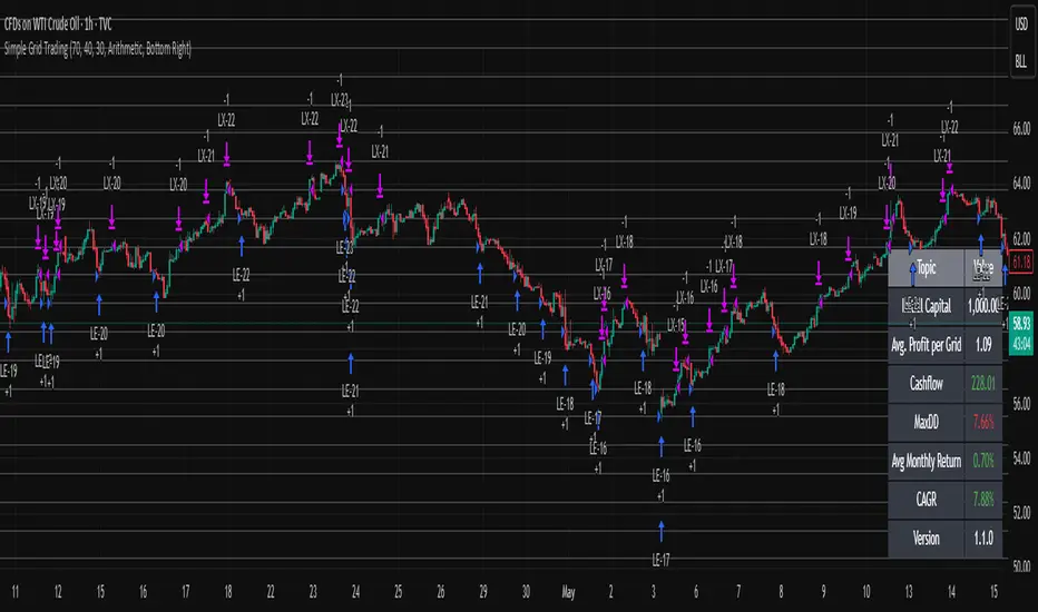
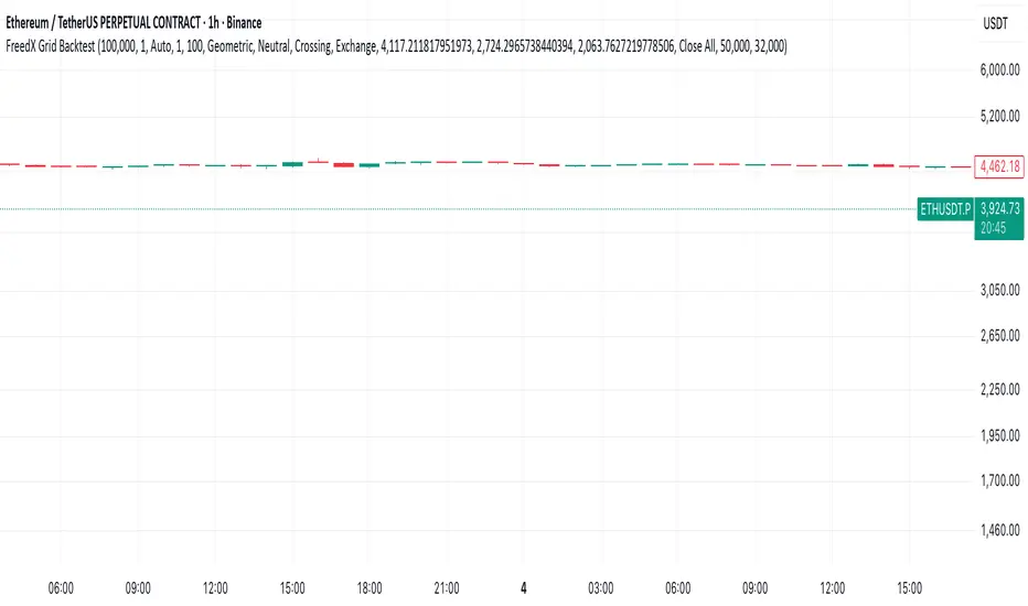
Simple Grid Trading v1.0 [PUCHON]Simple Grid Trading v1.0
Overview
This is a Long-Only Grid Trading Strategy developed in Pine Script v6 for TradingView. It is designed to profit from market volatility by placing a series of Buy Limit orders at predefined price levels. As the price drops, the strategy accumulates positions. As the price rises, it sells these positions at a profit.
Features
Grid Types : Supports both Arithmetic (equal price spacing) and Geometric (equal percentage spacing) grids.
Flexible Order Management : Uses strategy.order for precise control and prevents duplicate orders at the same level.
Performance Dashboard : A real-time table displaying key metrics like Capital, Cashflow, and Drawdown.
Advanced Metrics : Includes Max Drawdown (MaxDD) , Avg Monthly Return , and CAGR calculations.
Customizable : Fully adjustable price range, grid lines, and lot size.
Dashboard Metrics
The dashboard (default: Bottom Right) provides a quick snapshot of the strategy's performance:
Initial Capital : The starting capital defined in the strategy settings.
Lot Size : The fixed quantity of assets purchased per grid level.
Avg. Profit per Grid : The average realized profit for each closed trade.
Cashflow : The total realized net profit (closed trades only).
MaxDD : Maximum Drawdown . The largest percentage drop in equity (realized + unrealized) from a peak.
Avg Monthly Return : The average percentage return generated per month.
CAGR : Compound Annual Growth Rate . The mean annual growth rate of the investment over the specified time period.
Strategy Settings (Inputs)
Grid Settings
Upper Price : The highest price level for the grid.
Lower Price : The lowest price level for the grid.
Number of Grid Lines : The total number of levels (lines) in the grid.
Grid Type :
Arithmetic: Distance between lines is fixed in price terms (e.g., $10, $20, $30).
Geometric: Distance between lines is fixed in percentage terms (e.g., 1%, 2%, 3%).
Lot Size : The fixed amount of the asset to buy at each level.
Dashboard Settings
Show Dashboard : Toggle to hide/show the performance table.
Position : Choose where the dashboard appears on the chart (e.g., Bottom Right, Top Left).
How It Works
Initialization : On the first bar, the script calculates the price levels based on your Upper/Lower price and Grid Type.
Entry Logic :
The strategy places Buy Limit orders at every grid level below the current price.
It checks if a position already exists at a specific level to avoid "stacking" multiple orders on the same line.
Exit Logic :
For every Buy order, a corresponding Sell Limit (Take Profit) order is placed at the next higher grid level.
MaxDD Calculation :
The script continuously tracks the highest equity peak.
It calculates the drawdown on every bar (including intra-bar movements) to ensure accuracy.
Displayed as a percentage (e.g., 5.25%).
Disclaimer
This script is for educational and backtesting purposes only. Grid trading involves significant risk, especially in strong trending markets where the price may move outside your grid range. Always use proper risk management.
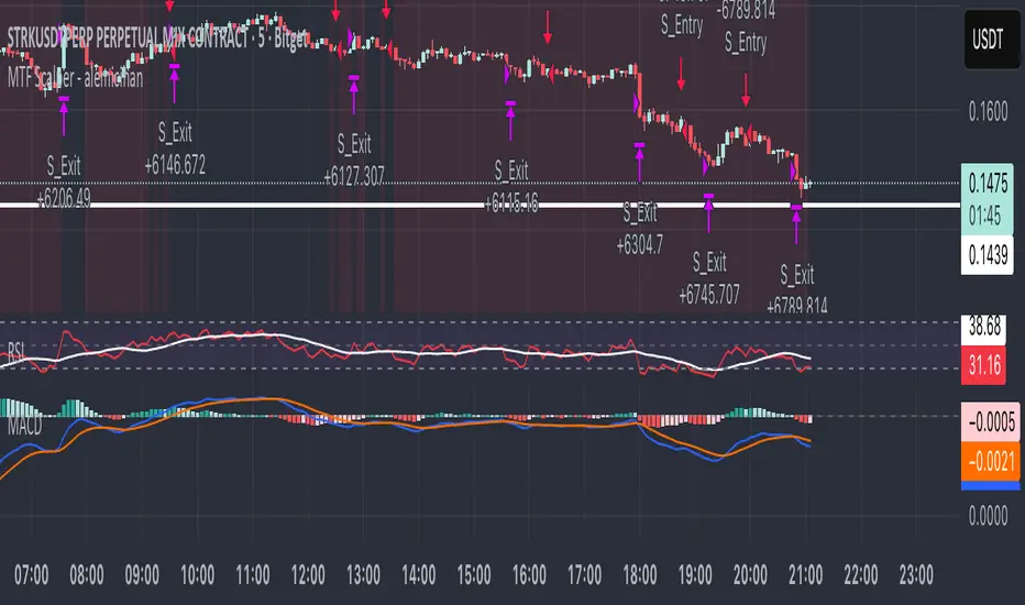
MTF Scalper - alemicihanMulti-Timeframe Scalper Strategy: Aligning the Big Picture for Quick Gains
This article presents a robust futures trading strategy designed for high-frequency scalping in the crypto market. It’s built on the principle of minimizing risk by ensuring that short-term entries are always aligned with the dominant, higher-timeframe trend.
The Core Concept: Alignment is Key
A Balanced Trend Follower approach, now refined for rapid scalping, uses a Multi-Timeframe (MTF) confirmation system to filter out market noise and increase the probability of a successful trade.
The strategy operates on a Low Timeframe (LTF) chart (e.g., 3m, 5m, or 15m) but only executes trades if the direction is validated by three Higher Timeframes (HTF).
ComponentPurposeFunctionHTF (D, 4h, 1h) EMA => Trend Confirmation =>Checks if the current price is above/below all three Exponential Moving Averages (EMA 20). This provides a strong directional bias.
LTF (5m) Stochastic RSI => Momentum Entry => Generates the actual buy/sell signal by spotting a swift crossover, indicating fresh momentum in the direction of the confirmed HTF trend.
How The Signal Is Generated
Trend Alignment: The system first confirms the trend. If the price is trading above the Daily, 4-Hour, and 1-Hour EMAs, the market is deemed to be in a Strong LONG Trend. Only LONG signals are permitted.
Momentum Trigger: Once the trend is confirmed, a Long Signal is generated only when the Stochastic K-Line crosses above the D-Line, indicating a momentum shift (a pullback ending) towards the main trend direction.
Short Signal: The inverse logic applies to the Short Trend confirmation and entry signal.
Mandatory Risk Management: ATR-Based Exit
Given the high leverage nature of futures and scalping, static Stop-Loss (SL) and Take-Profit (TP) levels are inefficient. This strategy uses the Average True Range (ATR) indicator to dynamically set profit and loss targets based on current market volatility.
Stop Loss (SL): Set dynamically at 1.5 x ATR below (for long) or above (for short) the entry price. This gives the trade enough room to breathe without risking excessive capital.
Take Profit (TP): Set dynamically at 3.0 x ATR, establishing a robust Risk-to-Reward Ratio of 1:2.
Final Thoughts on Testing
This sophisticated approach combines the reliability of MTF analysis with the speed of momentum indicators. However, data analysis is key. Backtesting these parameters (EMA, ATR Multipliers, RSI/Stochastic lengths) on your chosen asset (like BTC/USDT or ETH/USDT) and timeframe is crucial to achieving optimal performance.
HPAS mean reversion strategy testerTakes Krown HPAS values hardcoded and simulates longs and short with configurable standard deviation multiplier TP/SL. Best used on lower timeframes

Pivot Fib 4H — EAStrategy uses the pivot standard to open position, it has well define entry and exit point with SL, it also has a proper money management plan, maximum 4 trades a day, each trade risk 0.5% of the account, I have it EA version of it also.

Any Strategy BacktestA simple script for backtesting your strategies with TP and SL settings. For this to work, your indicators must have sources for long and short conditions.

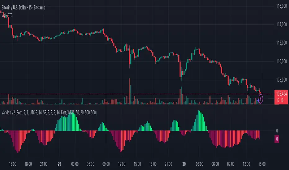
Vandan V2Vandan V2 is an automated trading strategy for NQ1! (E-mini Nasdaq-100) based on short-term mean reversion with dynamic risk control. It combines volatility filters and overbought/oversold signals to capture local market imbalances.
Backtested from 2015 to 2025, it achieved a +730% total return, Profit Factor of 1.40, max drawdown of only 1.61%, and over 106,000 trades. Designed for systematic scalping or intraday arbitrage with a limit of 3 simultaneous contracts.

Vandan V2Vandan V2 is an automated trend-following strategy for NASDAQ E-mini Futures (NQ1!).
It uses multi-timeframe momentum and volatility filters to identify high-probability entries.
Includes dynamic risk management and trailing logic optimized for intraday trading.
Master Trend Strategy - by jake_thebossMaster Trend Strategy
This strategy combines multiple technical indicators to identify high-probability trend entries across all asset classes.
Core Signal Logic:
Entry triggered when EMA 4 crosses above/below EMA 5
Confirmation required from RSI (>50 for long, <50 for short)
Price must be above/below key moving averages: EMA 21, SMA 50, EMA 55, EMA 89, and EMA 750
Additional confirmation from Stochastic (>52 bullish, <48 bearish) or EMA 89 breakout or VWAP cross
Key Features:
VWAP filter: Only takes bullish signals above VWAP and bearish signals below VWAP
Optional pyramiding: Allows multiple entries in the same direction (up to 200 orders)
Individual stop loss and take profit management for each pyramid level
Time filter: Customizable trading hours with timezone offset
Risk management: Adjustable stop loss (default 0.3%) and take profit (default 0.6%)
Visualization:
Entry, stop loss, and take profit levels drawn as horizontal lines
Customizable signal markers (triangles) for bull/bear entries
Optional EMA overlay display
The strategy is designed for trend-following on lower timeframes, with strict multi-indicator confirmation to filter out false signals.

Squeeze Backtest by Shaqi v2.0Script to backtest price squeeze's. Works on long and short directions

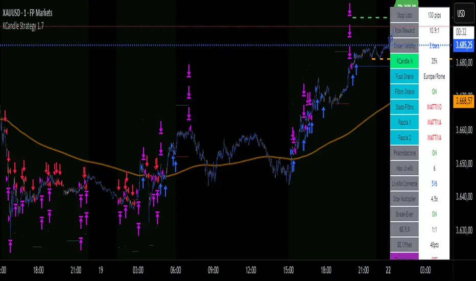
KCandle Strategy 1.0# KCandle Strategy 1.0 - Trading Strategy Description
## Overview
The **KCandle Strategy** is an advanced Pine Script trading system based on bullish and bearish engulfing candlestick patterns, enhanced with sophisticated risk management and position optimization features.
## Core Logic
### Entry Signal Generation
- **Pattern Recognition**: Detects bullish and bearish engulfing candlestick formations
- **EMA Filter**: Uses a customizable EMA (default 25) to filter trades in the direction of the trend
- **Entry Levels**:
- **Long entries** at 25% of the candlestick range from the low
- **Short entries** at 75% of the candlestick range from the low
- **Signal Validation**: Orange candlesticks indicate valid setup conditions
### Risk Management System
#### 1. **Stop Loss & Take Profit**
- Configurable stop loss in pips
- Risk-reward ratio setting (default 2:1)
- Visual representation with colored lines and labels
#### 2. **Break-Even Management**
- Automatically moves stop loss to break-even when specified R:R is reached
- Customizable break-even offset for added protection
- Prevents losing trades after reaching profitability
#### 3. **Trailing Stop System**
- **Activation Trigger**: Activates when position reaches specified R:R level
- **Distance Control**: Maintains trailing stop at defined distance from entry
- **Step Management**: Moves stop loss forward in incremental R steps
- **Dynamic Protection**: Locks in profits while allowing for continued upside
### Advanced Features
#### Position Management
- **Pyramiding Support**: Optional multiple position entries with size reduction
- **Order Expiration**: Pending orders automatically cancel after specified bars
- **Position Sizing**: Percentage-based allocation with pyramid level adjustments
#### Visual Interface
- **Real-time Monitoring**: Comprehensive information panel with all strategy metrics
- **Historical Tracking**: Visual representation of past trades and levels
- **Color-coded Indicators**: Different colors for break-even, trailing, and standard stops
- **Debug Options**: Optional labels for troubleshooting and optimization
## Key Parameters
### Basic Settings
- **EMA Length**: Trend filter period
- **Stop Loss**: Risk per trade in pips
- **Risk/Reward**: Target profit ratio
- **Order Validity**: Duration of pending orders
### Risk Management
- **Break-Even R:R**: Profit level to trigger break-even
- **Trailing Activation**: R:R level to start trailing
- **Trailing Distance**: Stop distance from entry when trailing
- **Trailing Step**: Increment for stop loss advancement
## Strategy Benefits
1. **Objective Entry Signals**: Based on proven candlestick patterns
2. **Trend Alignment**: EMA filter ensures trades align with market direction
3. **Robust Risk Control**: Multiple layers of protection (SL, BE, Trailing)
4. **Profit Optimization**: Trailing stops maximize winning trade potential
5. **Flexibility**: Extensive customization options for different market conditions
6. **Visual Clarity**: Complete visual feedback for trade management
## Ideal Use Cases
- **Swing Trading**: Medium-term positions with trend-following approach
- **Breakout Trading**: Capturing momentum from engulfing patterns
- **Risk-Conscious Trading**: Suitable for traders prioritizing capital preservation
- **Multi-Timeframe**: Adaptable to various timeframes and instruments
---
*The KCandle Strategy combines traditional technical analysis with modern risk management techniques, providing traders with a comprehensive tool for systematic market participation.*
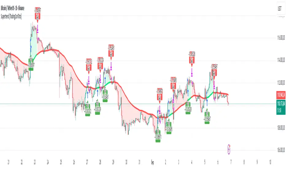
Supertrend [TradingConToto]Supertrend — ADX/DI + EMA Gap + Breakout (with Mobile UI)
What makes it original
Supertrend combines trend strength (ADX/DI), multi-timeframe bias (EMA63 and EMA 200D equivalent), a structural filter based on the distance between EMA2400 and EMA4800 expressed in ATR units, and a momentum confirmation through a previous high breakout.
This is not a random mashup — it’s a sequence of filters designed to reduce trades in ranging markets and prioritize mature trends:
Direction: +DI > -DI (trend led by buyers).
Strength: ADX > mean(ADX) (avoids weak, choppy phases).
Short-term bias: Close > EMA63.
Long-term bias: Close > EMA4800 ≈ EMA200 daily on H1.
Momentum: Close > High (immediate breakout).
Structure: (EMA2400 − EMA4800) > k·ATR (ensures separation in ATR units, filters out flat phases).
Entries & exits
Entry: when all six conditions are met and no open position exists.
Exit: if +DI < -DI or Close < EMA63.
Visuals: EMA63 is painted green while in position and red otherwise, with a supertrend-style band; “BUY” labels appear below the green band and “SELL” labels above the red band.
UI: includes a compact table (mobile-friendly) showing the state of each condition.
Default parameters used in this publication
Initial capital: 10,000
Position size: 10% of equity (≤10% per trade is considered sustainable).
Commission: 0.01% per side (adjust to your broker/market).
Slippage: 1 tick
Pyramiding: 0 (only one position at a time)
Adjust commission/slippage to match your market. For US equities, commissions are often per share; for spot crypto, 0.10–0.20% total is common. I publish with 0.01% per side as a conservative example to avoid overestimating results.
Recommended backtest dataset
Timeframe: H1
Multi-cycle window (e.g. 2015–today)
Symbols with high liquidity (e.g. NASDAQ-100 large caps, or BTC/ETH spot) to generate 100+ trades. Avoid cherry-picked short windows.
Why each filter matters
+DI > -DI + ADX > mean: reduce counter-trend trades and weak signals.
Close > EMA63 + Close > EMA4800: enforce trend alignment in short and long horizons.
Breakout High : requires immediate momentum, avoids early entries.
EMA gap in ATR units: blocks flat or compressed structures where EMA200D aligns with price.
Limitations
The breakout filter may skip healthy pullbacks; the design prioritizes continuation over perfect entry price.
No fixed trailing stop/TP; exits depend on trend degradation via DI/EMA63.
Results vary with real costs (commissions, slippage, funding). Adjust defaults to your broker.
How to use
Apply it on a clean chart (no other indicators when publishing).
Keep in mind the default parameters above; if you change them, mention it in your notes and use the same values in the Strategy Tester.
Ensure your dataset produces 100+ trades for statistical validity.
Lunar calendar day Crypto Trading StrategyLunar calendar day Crypto Trading Strategy
This strategy explores the potential impact of the lunar calendar on cryptocurrency price cycles.
It implements a simple but unconventional rule:
Buy on the 5th day of each lunar month
Sell on the 26th day of the lunar month
No trades between January 1 (solar) and Lunar New Year’s Day (holiday buffer period)
Research background
Several academic studies have investigated the influence of lunar cycles on financial markets. Their findings suggest:
Returns tend to be higher around the full moon compared to the new moon.
Periods between the full moon and the waning phase often show stronger average returns than the waxing phase.
This strategy combines those observations into a practical implementation by testing fixed entry (lunar day 5) and exit (lunar day 26) points, while excluding the transition period from solar New Year to Lunar New Year, effectively capturing mid-month lunar effects.
How it works
The script includes a custom lunar date calculation function, reconstructing lunar months and days for each year (2020–2026).
On lunar day 5, the strategy opens a long position with 100% of equity.
On lunar day 26, the strategy closes the position.
No trades are executed between Jan 1 and Lunar New Year’s Day.
All trades include:
Commission: 0.1%
Slippage: 3 ticks
Position sizing uses the entire equity (100%) for simplicity, but this is not recommended for live trading.
Why this is original
Unlike mashups of built-in indicators, this script:
Implements a full lunar calendar system inside Pine Script.
Translates academic findings on lunar effects into an applied backtest.
Adds a realistic trading filter (holiday gap) based on cultural/seasonal calendar rules.
Provides researchers and traders with a framework to explore non-traditional, time-based signals.
Notes
This is an experimental, research-oriented strategy, not financial advice.
Results are highly dependent on the chosen period (2020–2026).
Using 100% equity per trade is for simplification only and is not a viable money management practice.
The purpose is to investigate whether cyclical patterns linked to lunar time can provide any statistical edge in ETHUSDT.

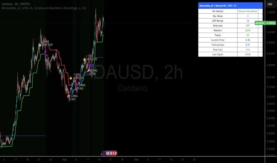
Mutanabby_AI | ATR+ | Trend-Following StrategyThis document presents the Mutanabby_AI | ATR+ Pine Script strategy, a systematic approach designed for trend identification and risk-managed position entry in financial markets. The strategy is engineered for long-only positions and integrates volatility-adjusted components to enhance signal robustness and trade management.
Strategic Design and Methodological Basis
The Mutanabby_AI | ATR+ strategy is constructed upon a foundation of established technical analysis principles, with a focus on objective signal generation and realistic trade execution.
Heikin Ashi for Trend Filtering: The core price data is processed via Heikin Ashi (HA) methodology to mitigate transient market noise and accentuate underlying trend direction. The script offers three distinct HA calculation modes, allowing for comparative analysis and validation:
Manual Calculation: Provides a transparent and deterministic computation of HA values.
ticker.heikinashi(): Utilizes TradingView's built-in function, employing confirmed historical bars to prevent repainting artifacts.
Regular Candles: Allows for direct comparison with standard OHLC price action.
This multi-methodological approach to trend smoothing is critical for robust signal generation.
Adaptive ATR Trailing Stop: A key component is the Average True Range (ATR)-based trailing stop. ATR serves as a dynamic measure of market volatility. The strategy incorporates user-defined parameters (
Key Value and ATR Period) to calibrate the sensitivity of this trailing stop, enabling adaptation to varying market volatility regimes. This mechanism is designed to provide a dynamic exit point, preserving capital and locking in gains as a trend progresses.
EMA Crossover for Signal Generation: Entry and exit signals are derived from the interaction between the Heikin Ashi derived price source and an Exponential Moving Average (EMA). A crossover event between these two components is utilized to objectively identify shifts in momentum, signaling potential long entry or exit points.
Rigorous Stop Loss Implementation: A critical feature for risk mitigation, the strategy includes an optional stop loss. This stop loss can be configured as a percentage or fixed point deviation from the entry price. Importantly, stop loss execution is based on real market prices, not the synthetic Heikin Ashi values. This design choice ensures that risk management is grounded in actual market liquidity and price levels, providing a more accurate representation of potential drawdowns during backtesting and live operation.
Backtesting Protocol: The strategy is configured for realistic backtesting, employing fill_orders_on_standard_ohlc=true to simulate order execution at standard OHLC prices. A configurable Date Filter is included to define specific historical periods for performance evaluation.
Data Visualization and Metrics: The script provides on-chart visual overlays for buy/sell signals, the ATR trailing stop, and the stop loss level. An integrated information table displays real-time strategy parameters, current position status, trend direction, and key price levels, facilitating immediate quantitative assessment.
Applicability
The Mutanabby_AI | ATR+ strategy is particularly suited for:
Cryptocurrency Markets: The inherent volatility of assets such as #Bitcoin and #Ethereum makes the ATR-based trailing stop a relevant tool for dynamic risk management.
Systematic Trend Following: Individuals employing systematic methodologies for trend capture will find the objective signal generation and rule-based execution aligned with their approach.
Pine Script Developers and Quants: The transparent code structure and emphasis on realistic backtesting provide a valuable framework for further analysis, modification, and integration into broader quantitative models.
Automated Trading Systems: The clear, deterministic entry and exit conditions facilitate integration into automated trading environments.
Implementation and Evaluation
To evaluate the Mutanabby_AI | ATR+ strategy, apply the script to your chosen chart on TradingView. Adjust the input parameters (Key Value, ATR Period, Heikin Ashi Method, Stop Loss Settings) to observe performance across various asset classes and timeframes. Comprehensive backtesting is recommended to assess the strategy's historical performance characteristics, including profitability, drawdown, and risk-adjusted returns.
I'd love to hear your thoughts, feedback, and any optimizations you discover! Drop a comment below, give it a like if you find it useful, and share your results.
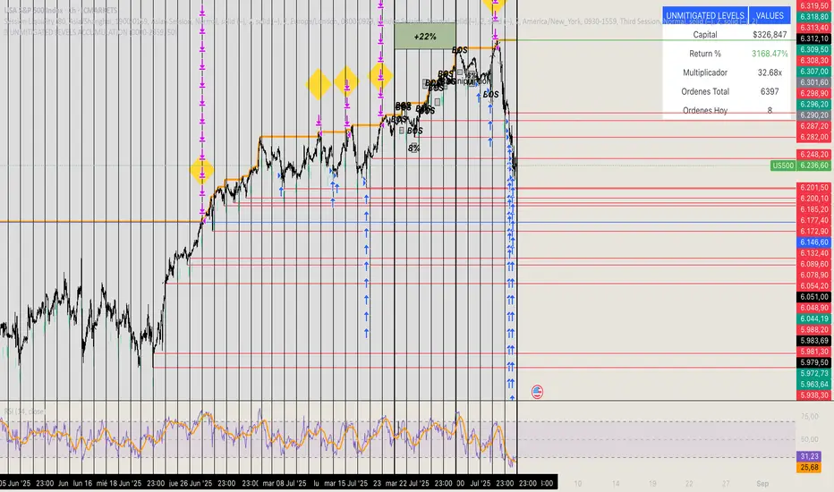
🏆 UNMITIGATED LEVELS ACCUMULATIONPDH TO ATH RISK FREE
All the PDL have a buy limit which starts at 0.1 lots which will duplicate at the same time the capital incresases. All of the buy limits have TP in ATH for max reward.
safa bot alertGood trading for everying and stuff that very gfood and stuff please let me puibisjertpa 9uihthsi fuckitgn code

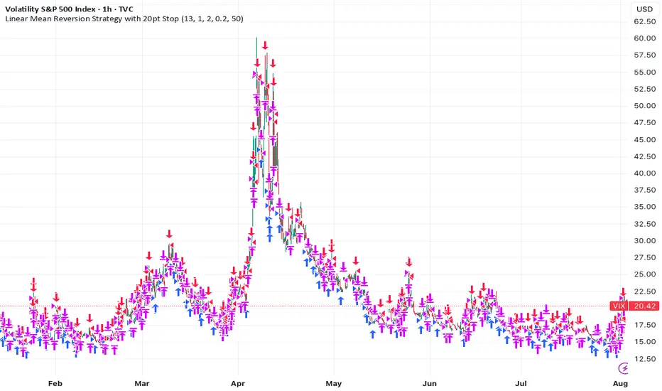
Linear Mean Reversion Strategy📘 Strategy Introduction: Linear Mean Reversion with Fixed Stop
This strategy implements a simple yet powerful mean reversion model that assumes price tends to oscillate around a dynamic average over time. It identifies statistically significant deviations from the moving average using a z-score, and enters trades expecting a return to the mean.
🧠 Core Logic:
A z-score is calculated by comparing the current price to its moving average, normalized by standard deviation, over a user-defined half-life window.
Trades are entered when the z-score crosses a threshold (e.g., ±1), signaling overbought or oversold conditions.
The strategy exits positions either when price reverts back near the mean (z-score close to 0), or if a fixed stop loss of 100 points is hit, whichever comes first.
⚙️ Key Features:
Dynamic mean and volatility estimation using moving average and standard deviation
Configurable z-score thresholds for entry and exit
Position size scaling based on z-score magnitude
Fixed stop loss to control risk and avoid prolonged drawdowns
🧪 Use Case:
Ideal for range-bound markets or assets that exhibit stationary behavior around a mean, this strategy is especially useful on assets with mean-reverting characteristics like currency pairs, ETFs, or large-cap stocks. It is best suited for traders looking for short-term reversions rather than long-term trends.
EUR/USD Multi-Layer Statistical Regression StrategyStrategy Overview
This advanced EUR/USD trading system employs a triple-layer linear regression framework with statistical validation and ensemble weighting. It combines short, medium, and long-term regression analyses to generate high-confidence directional signals while enforcing strict risk controls.
Core Components
Multi-Layer Regression Engine:
Parallel regression analysis across 3 customizable timeframes (short/medium/long)
Projects future price values using prediction horizons
Statistical significance filters (R-squared, correlation, slope thresholds)
Signal Validation System:
Lookback validation tests historical prediction accuracy
Ensemble weighting of layer signals (adjustable influence per timeframe)
Confidence scoring combining statistical strength, layer agreement, and validation accuracy
Risk Management:
Position sizing scaled by signal confidence (1%-100% of equity)
Daily loss circuit breaker (halts trading at user-defined threshold)
Forex-tailored execution (pip slippage, percentage-based commissions)
Visual Intelligence:
Real-time regression line plots (3 layered colors)
Projection markers for short-term forecasts
Background coloring for market bias indication
Comprehensive statistics dashboard (R-squared metrics, validation scores, P&L)
Key Parameters
Category Settings
Regression Short/Med/Long lengths (20/50/100 bars)
Statistics Min R² (0.65), Correlation (0.7), Slope (0.0001)
Validation 30-bar lookback, 10-bar projection
Risk Controls 50% position size, 12% daily loss limit, 75% confidence threshold
Trading Logic
Entries require:
Ensemble score > |0.5|
Confidence > threshold
Short & medium-term significance
Active daily loss limit not breached
Exits triggered by:
Opposite high-confidence signals
Daily loss limit violation (emergency exit)
The strategy blends quantitative finance techniques with practical trading safeguards, featuring a self-optimizing design where signal quality directly impacts position sizing. The visual dashboard provides real-time feedback on model performance and market conditions.

CCI-MACD Strategy 4.2
I cerchi si basano sull'oscillatore CCI (Commodity Channel Index).
L’indicatore CCI ci permette di osservare se il livello attuale del prezzo è particolarmente al di sopra o al di sotto di una certa media mobile, avente un numero di periodi scelto da noi.
Più la deviazione dal prezzo medio nel breve termine è forte, e maggiormente l’indicatore si allontanerà dallo 0: verso l’alto in caso di uptrend, o verso il basso in caso di downtrend.
Il segnale viene dato quando il valore del CCI supera la linea dello zero.
Il tutto è filtrato con un altro indicatore, il MACD, acronimo di "Moving Average Convergence Divergence", usato per identificare cambiamenti nel momentum del prezzo.
The circles are based on the CCI (Commodity Channel Index) oscillator.
The CCI indicator allows us to observe whether the current price level is significantly above or below a certain moving average, with a number of periods chosen by us.
The greater the deviation from the short-term average price, the further the indicator will deviate from 0: upwards in the case of an uptrend, or downwards in the case of a downtrend.
The signal is given when the CCI value crosses the zero line.
This is all filtered through another indicator, the MACD, which stands for "Moving Average Convergence Divergence," used to identify changes in price momentum.

Eliora Gold 1min (Heikin Ashi)Eliora -focused trading strategy designed for anything on the 1-minute timeframe using Heikin Ashi candles. This mode combines advanced market logic with structured risk management to deliver smooth, disciplined trade execution.
Key Features:
✅ Trend Confirmation – Aligns with dominant market direction for higher accuracy.
✅ ATR-Based Volatility Filter – Avoids high-risk conditions and chaotic price action.
✅ Candle Strength Logic – Filters weak setups, focusing on strong momentum.
✅ Balanced Risk/Reward – Calculates stop-loss and take-profit dynamically for consistent results.
✅ Cooldown & Overtrade Protection – Limits frequency to maintain trade quality.
This version of Eliora is built for scalpers and intraday traders seeking high-probability entries with graceful exits.