McClellan A-D Volume Integration ModelThe strategy integrates the McClellan A-D Oscillator with an adjustment based on the Advance/Decline (A-D) volume data. The McClellan Oscillator is calculated by taking the difference between the short-term and long-term exponential moving averages (EMAs) of the A-D line. This strategy introduces an enhancement where the A-D volume (the difference between the advancing and declining volume) is factored in to adjust the oscillator value.
Inputs:
• ema_short_length: The length for the short-term EMA of the A-D line.
• ema_long_length: The length for the long-term EMA of the A-D line.
• osc_threshold_long: The threshold below which the oscillator must drop for an entry signal to trigger.
• exit_periods: The number of periods after which the position is closed.
• Data Sources:
• ad_advance and ad_decline are the data sources for advancing and declining issues, respectively.
• vol_advance and vol_decline are the volume data for the advancing and declining issues. If volume data is unavailable, it defaults to na (Not Available), and the fallback logic ensures that the strategy continues to function.
McClellan Oscillator with Volume Adjustment:
• The A-D line is calculated by subtracting the declining issues from the advancing issues. Then, the volume difference is applied to this line, creating a “weighted” A-D line.
• The short and long EMAs are calculated for the weighted A-D line to generate the McClellan Oscillator.
Entry Condition:
• The strategy looks for a reversal signal, where the oscillator falls below the threshold and then rises above it again. The condition is designed to trigger a long position when this reversal happens.
Exit Condition:
• The position is closed after a set number of periods (exit_periods) have passed since the entry.
Plotting:
• The McClellan Oscillator and the threshold are plotted on the chart for visual reference.
• Entry and exit signals are highlighted with background colors to make the signals more visible.
Scientific Background:
The McClellan A-D Oscillator is a popular market breadth indicator developed by Sherman and Marian McClellan. It is used to gauge the underlying strength of a market by analyzing the difference between the number of advancing and declining stocks. The oscillator is typically calculated using exponential moving averages (EMAs) of the A-D line, with the idea being that crossovers of these EMAs indicate potential changes in the market’s direction.
The integration of A-D volume into this model adds another layer of analysis, as volume is often considered a leading indicator of price movement. By factoring in volume, the strategy becomes more sensitive to not just the number of advancing or declining stocks but also how significant those movements are based on trading volume, as discussed in Schwager, J. D. (1999). Technical Analysis of the Financial Markets. This enhanced version aims to capture stronger and more sustainable trends in the market, helping to filter out false signals.
Additionally, volume analysis is often used to confirm price movements, as described in Wyckoff, R. (1931). The Day Trading System. Therefore, incorporating the volume of advancing and declining stocks in the McClellan Oscillator offers a more robust signal for trading decisions.
Statistics

Z-Strike RecoveryThis strategy utilizes the Z-Score of daily changes in the VIX (Volatility Index) to identify moments of extreme market panic and initiate long entries. Scientific research highlights that extreme volatility levels often signal oversold markets, providing opportunities for mean-reversion strategies.
How the Strategy Works
Calculation of Daily VIX Changes:
The difference between today’s and yesterday’s VIX closing prices is calculated.
Z-Score Calculation:
The Z-Score quantifies how far the current change deviates from the mean (average), expressed in standard deviations:
Z-Score=(Daily VIX Change)−MeanStandard Deviation
Z-Score=Standard Deviation(Daily VIX Change)−Mean
The mean and standard deviation are computed over a rolling period of 16 days (default).
Entry Condition:
A long entry is triggered when the Z-Score exceeds a threshold of 1.3 (adjustable).
A high positive Z-Score indicates a strong overreaction in the market (panic).
Exit Condition:
The position is closed after 10 periods (days), regardless of market behavior.
Visualizations:
The Z-Score is plotted to make extreme values visible.
Horizontal threshold lines mark entry signals.
Bars with entry signals are highlighted with a blue background.
This strategy is particularly suitable for mean-reverting markets, such as the S&P 500.
Scientific Background
Volatility and Market Behavior:
Studies like Whaley (2000) demonstrate that the VIX, known as the "fear gauge," is highly correlated with market panic phases. A spike in the VIX is often interpreted as an oversold signal due to excessive hedging by investors.
Source: Whaley, R. E. (2000). The investor fear gauge. Journal of Portfolio Management, 26(3), 12-17.
Z-Score in Financial Strategies:
The Z-Score is a proven method for detecting statistical outliers and is widely used in mean-reversion strategies.
Source: Chan, E. (2009). Quantitative Trading. Wiley Finance.
Mean-Reversion Approach:
The strategy builds on the mean-reversion principle, which assumes that extreme market movements tend to revert to the mean over time.
Source: Jegadeesh, N., & Titman, S. (1993). Returns to Buying Winners and Selling Losers: Implications for Stock Market Efficiency. Journal of Finance, 48(1), 65-91.

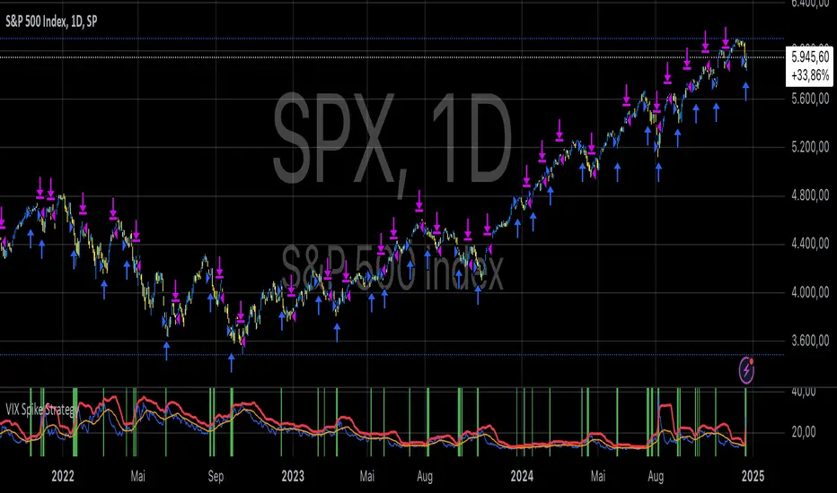
VIX Spike StrategyThis script implements a trading strategy based on the Volatility Index (VIX) and its standard deviation. It aims to enter a long position when the VIX exceeds a certain number of standard deviations above its moving average, which is a signal of a volatility spike. The position is then exited after a set number of periods.
VIX Symbol (vix_symbol): The input allows the user to specify the symbol for the VIX index (typically "CBOE:VIX").
Standard Deviation Length (stddev_length): The number of periods used to calculate the standard deviation of the VIX. This can be adjusted by the user.
Standard Deviation Multiplier (stddev_multiple): This multiplier is used to determine how many standard deviations above the moving average the VIX must exceed to trigger a long entry.
Exit Periods (exit_periods): The user specifies how many periods after entering the position the strategy will exit the trade.
Strategy Logic:
Data Loading: The script loads the VIX data, both for the current timeframe and as a rescaled version for calculation purposes.
Standard Deviation Calculation: It calculates both the moving average (SMA) and the standard deviation of the VIX over the specified period (stddev_length).
Entry Condition: A long position is entered when the VIX exceeds the moving average by a specified multiple of its standard deviation (calculated as vix_mean + stddev_multiple * vix_stddev).
Exit Condition: After the position is entered, it will be closed after the user-defined number of periods (exit_periods).
Visualization:
The VIX is plotted in blue.
The moving average of the VIX is plotted in orange.
The threshold for the VIX, which is the moving average plus the standard deviation multiplier, is plotted in red.
The background turns green when the entry condition is met, providing a visual cue.
Sources:
The VIX is often used as a measure of market volatility, with high values indicating increased uncertainty in the market.
Standard deviation is a statistical measure of the variability or dispersion of a set of data points. In financial markets, it is used to measure the volatility of asset prices.
References:
Bollerslev, T. (1986). "Generalized Autoregressive Conditional Heteroskedasticity." Journal of Econometrics.
Black, F., & Scholes, M. (1973). "The Pricing of Options and Corporate Liabilities." Journal of Political Economy.
R-based Strategy Template [Daveatt]Have you ever wondered how to properly track your trading performance based on risk rather than just profits?
This template solves that problem by implementing R-multiple tracking directly in TradingView's strategy tester.
This script is a tool that you must update with your own trading entry logic.
Quick notes
Before we dive in, I want to be clear: this is a template focused on R-multiple calculation and visualization.
I'm using a basic RSI strategy with dummy values just to demonstrate how the R tracking works. The actual trading signals aren't important here - you should replace them with your own strategy logic.
R multiple logic
Let's talk about what R-multiple means in practice.
Think of R as your initial risk per trade.
For instance, if you have a $10,000 account and you're risking 1% per trade, your 1R would be $100.
A trade that makes twice your risk would be +2R ($200), while hitting your stop loss would be -1R (-$100).
This way of measuring makes it much easier to evaluate your strategy's performance regardless of account size.
Whenever the SL is hit, we lose -1R
Proof showing the strategy tester whenever the SL is hit: i.imgur.com
The magic happens in how we calculate position sizes.
The script automatically determines the right position size to risk exactly your specified percentage on each trade.
This is done through a simple but powerful calculation:
risk_amount = (strategy.equity * (risk_per_trade_percent / 100))
sl_distance = math.abs(entry_price - sl_price)
position_size = risk_amount / (sl_distance * syminfo.pointvalue)
Limitations with lower timeframe gaps
This ensures that if your stop loss gets hit, you'll lose exactly the amount you intended to risk. No more, no less.
Well, could be more or less actually ... let's assume you're trading futures on a 15-minute chart but in the 1-minute chart there is a gap ... then your 15 minute SL won't get filled and you'll likely to not lose exactly -1R
This is annoying but it can't be fixed - and that's how trading works anyway.
Features
The template gives you flexibility in how you set your stop losses. You can use fixed points, ATR-based stops, percentage-based stops, or even tick-based stops.
Regardless of which method you choose, the position sizing will automatically adjust to maintain your desired risk per trade.
To help you track performance, I've added a comprehensive statistics table in the top right corner of your chart.
It shows you everything you need to know about your strategy's performance in terms of R-multiples: how many R you've won or lost, your win rate, average R per trade, and even your longest winning and losing streaks.
Happy trading!
And remember, measuring your performance in R-multiples is one of the most classical ways to evaluate and improve your trading strategies.
Daveatt
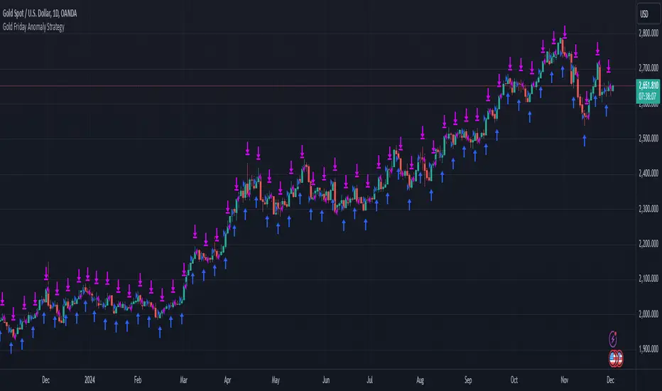
Gold Friday Anomaly StrategyThis script implements the " Gold Friday Anomaly Strategy ," a well-known historical trading strategy that leverages the gold market's behavior from Thursday evening to Friday close. It is a backtesting-focused strategy designed to assess the historical performance of this pattern. Traders use this anomaly as it captures a recurring market tendency observed over the years.
What It Does:
Entry Condition: The strategy enters a long position at the beginning of the Friday trading session (Thursday evening close) within the defined backtesting period.
Exit Condition: Friday evening close.
Backtesting Controls: Allows users to set custom backtesting periods to evaluate strategy performance over specific date ranges.
Key Features:
Custom Backtest Periods: Easily configurable inputs to set the start and end date of the backtesting range.
Fixed Slippage and Commission Settings: Ensures realistic simulation of trading conditions.
Process Orders on Close: Backtesting is optimized by processing orders at the bar's close.
Important Notes:
Backtesting Only: This script is intended purely for backtesting purposes. Past performance is not indicative of future results.
Live Trading Recommendations: For live trading, it is highly recommended to use limit orders instead of market orders, especially during evening sessions, as market order slippage can be significant.
Default Settings:
Entry size: 10% of equity per trade.
Slippage: 1 tick.
Commission: 0.05% per trade.
BTC Seasonality Strategy (Weekly)This strategy identifies potential weekend opportunities in Bitcoin (BTC) markets by leveraging the concept of seasonality, entering a position at a predefined time and day, and exiting at a specified time and day.
Key Features
Customizable Time and Day Selection:
Users can select the entry and exit days and corresponding times (in EST).
Directional Flexibility:
The strategy allows traders to choose between long or short positions.
TradingView Compliance:
The script adheres to TradingView's house rules, avoids overly complex conditions, and provides clear user-configurable inputs.
How It Works
The script determines the current weekday and hour in EST, converting TradingView's UTC time for accurate comparisons.
If the current day and hour match the selected entry conditions, a trade (long or short) is opened.
The position is closed when the current day and hour match the specified exit conditions.
Theoretical Basis
Market Seasonality:
The concept of seasonality in financial markets refers to predictable patterns based on time, such as weekends or specific days of the week. Studies have shown that cryptocurrency markets exhibit unique trading behaviors during weekends due to reduced institutional activity and higher retail participation behavioral Biases**:
Retail traders often dominate weekend markets, potentially causing predictable inefficiencies .
Reverences**
Baur, D. G., Hong, K., & Lee, A. D. (2018). Bitcoin: Medium of exchange or speculative assets? Journal of International Financial Markets, Institutions and Money, 54, 177–189.
Urquhart, A. (2016). The inefficiency of Bitcoin. Economics Letters, 148, 80–82.

Global Index Spread RSI StrategyThis strategy leverages the relative strength index (RSI) to monitor the price spread between a global benchmark index (such as AMEX) and the currently opened asset in the chart window. By calculating the spread between these two, the strategy uses RSI to identify oversold and overbought conditions to trigger buy and sell signals.
Key Components:
Global Benchmark Index: The strategy compares the current asset with a predefined global index (e.g., AMEX) to measure relative performance. The choice of a global benchmark allows the trader to analyze the current asset's movement in the context of broader market trends.
Spread Calculation:
The spread is calculated as the percentage difference between the current asset's closing price and the global benchmark index's closing price:
Spread=Current Asset Close−Global Index CloseGlobal Index Close×100
Spread=Global Index CloseCurrent Asset Close−Global Index Close×100
This metric provides a measure of how the current asset is performing relative to the global index. A positive spread indicates the asset is outperforming the benchmark, while a negative spread signals underperformance.
RSI of the Spread: The RSI is then calculated on the spread values. The RSI is a momentum oscillator that ranges from 0 to 100 and is commonly used to identify overbought or oversold conditions in asset prices. An RSI below 30 is considered oversold, indicating a potential buying opportunity, while an RSI above 70 is overbought, suggesting that the asset may be due for a pullback.
Strategy Logic:
Entry Condition: The strategy enters a long position when the RSI of the spread falls below the oversold threshold (default 30). This suggests that the asset may have been oversold relative to the global benchmark and might be due for a reversal.
Exit Condition: The strategy exits the long position when the RSI of the spread rises above the overbought threshold (default 70), indicating that the asset may have become overbought and a price correction is likely.
Visual Reference:
The RSI of the spread is plotted on the chart for visual reference, making it easier for traders to monitor the relative strength of the asset in relation to the global benchmark.
Overbought and oversold levels are also drawn as horizontal reference lines (70 and 30), along with a neutral level at 50 to show market equilibrium.
Theoretical Basis:
The strategy is built on the mean reversion principle, which suggests that asset prices tend to revert to a long-term average over time. When prices move too far from this mean—either being overbought or oversold—they are likely to correct back toward equilibrium. By using RSI to identify these extremes, the strategy aims to profit from price reversals.
Mean Reversion: According to financial theory, asset prices oscillate around a long-term average, and any extreme deviation (overbought or oversold conditions) presents opportunities for price corrections (Poterba & Summers, 1988).
Momentum Indicators (RSI): The RSI is widely used in technical analysis to measure the momentum of an asset. Its application to the spread between the asset and a global benchmark allows for a more nuanced view of relative performance and potential turning points in the asset's price trajectory.
Practical Application:
This strategy works best in markets where relative strength is a key factor in decision-making, such as in equity indices, commodities, or forex markets. By assessing the performance of the asset relative to a global benchmark and utilizing RSI to identify extremes in price movements, the strategy helps traders to make more informed decisions based on potential mean reversion points.
While the "Global Index Spread RSI Strategy" offers a method for identifying potential price reversals based on relative strength and oversold/overbought conditions, it is important to recognize that no strategy is foolproof. The strategy assumes that the historical relationship between the asset and the global benchmark will hold in the future, but financial markets are subject to a wide array of unpredictable factors that can lead to sudden changes in price behavior.
Risk of False Signals:
The strategy relies heavily on the RSI to trigger buy and sell signals. However, like any momentum-based indicator, RSI can generate false signals, particularly in highly volatile or trending markets. In such conditions, the strategy may enter positions too early or exit too late, leading to potential losses.
Market Context:
The strategy may not account for macroeconomic events, news, or other market forces that could cause sudden shifts in asset prices. External factors, such as geopolitical developments, monetary policy changes, or financial crises, can cause a divergence between the asset and the global benchmark, leading to incorrect conclusions from the strategy.
Overfitting Risk:
As with any strategy that uses historical data to make decisions, there is a risk of overfitting the model to past performance. This could result in a strategy that works well on historical data but performs poorly in live trading conditions due to changes in market dynamics.
Execution Risks:
The strategy does not account for slippage, transaction costs, or liquidity issues, which can impact the execution of trades in real-market conditions. In fast-moving markets, prices may move significantly between order placement and execution, leading to worse-than-expected entry or exit prices.
No Guarantee of Profit:
Past performance is not necessarily indicative of future results. The strategy should be used with caution, and risk management techniques (such as stop losses and position sizing) should always be implemented to protect against significant losses.
Traders should thoroughly test and adapt the strategy in a simulated environment before applying it to live trades, and consider seeking professional advice to ensure that their trading activities align with their risk tolerance and financial goals.
References:
Poterba, J. M., & Summers, L. H. (1988). Mean Reversion in Stock Prices: Evidence and Implications. Journal of Financial Economics, 22(1), 27-59.

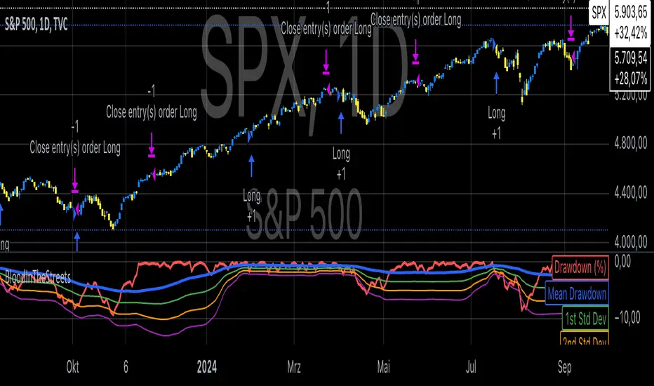
Buy When There's Blood in the Streets StrategyStatistical Analysis of Drawdowns in Stock Markets
Drawdowns, defined as the decline from a peak to a trough in asset prices, are an essential measure of risk and market dynamics. Their statistical properties provide insights into market behavior during extreme stress periods.
Distribution of Drawdowns: Research suggests that drawdowns follow a power-law distribution, implying that large drawdowns, while rare, are more frequent than expected under normal distributions (Sornette et al., 2003).
Impacts of Extreme Drawdowns: During significant drawdowns (e.g., financial crises), the average recovery time is significantly longer, highlighting market inefficiencies and behavioral biases. For example, the 2008 financial crisis led to a 57% drawdown in the S&P 500, requiring years to recover (Cont, 2001).
Using Standard Deviations: Drawdowns exceeding two or three standard deviations from their historical mean are often indicative of market overreaction or capitulation, creating contrarian investment opportunities (Taleb, 2007).
Behavioral Finance Perspective: Investors often exhibit panic-selling during drawdowns, leading to oversold conditions that can be exploited using statistical thresholds like standard deviations (Kahneman, 2011).
Practical Implications: Studies on mean reversion show that extreme drawdowns are frequently followed by periods of recovery, especially in equity markets. This underpins strategies that "buy the dip" under specific, statistically derived conditions (Jegadeesh & Titman, 1993).
References:
Sornette, D., & Johansen, A. (2003). Stock market crashes and endogenous dynamics.
Cont, R. (2001). Empirical properties of asset returns: stylized facts and statistical issues. Quantitative Finance.
Taleb, N. N. (2007). The Black Swan: The Impact of the Highly Improbable.
Kahneman, D. (2011). Thinking, Fast and Slow.
Jegadeesh, N., & Titman, S. (1993). Returns to Buying Winners and Selling Losers: Implications for Stock Market Efficiency.
BarRange StrategyHello,
This is a long-only, volatility-based strategy that analyzes the range of the previous bar (high - low).
If the most recent bar’s range exceeds a threshold based on the last X bars, a trade is initiated.
You can customize the lookback period, threshold value, and exit type.
For exits, you can choose to exit after X bars or when the close price exceeds the previous bar’s high.
The strategy is designed for instruments with a long-term upward-sloping curves, such as ES1! or NQ1!. It may not perform well on other instruments.
Commissions are set to $2.50 per side ($5.00 per round trip).
Recommended timeframes are 1h and higher. With adjustments to the lookback period and threshold, it could potentially achieve similar results on lower timeframes as well.

FTMO Rules MonitorFTMO Rules Monitor: Stay on Track with Your FTMO Challenge Goals
TLDR; You can test with this template whether your strategy for one asset would pass the FTMO challenges step 1 then step 2, then with real money conditions.
Passing a prop firm challenge is ... challenging.
I believe a toolkit allowing to test in minutes whether a strategy would have passed a prop firm challenge in the past could be very powerful.
The FTMO Rules Monitor is designed to help you stay within FTMO’s strict risk management guidelines directly on your chart. Whether you’re aiming for the $10,000 or the $200,000 account challenge, this tool provides real-time tracking of your performance against FTMO’s rules to ensure you don’t accidentally breach any limits.
NOTES
The connected indicator for this post doesn't matter.
It's just a dummy double supertrends (see below)
The strategy results for this script post does not matter as I'm posting a FTMO rules template on which you can connect any indicator/strategy.
//@version=5
indicator("Supertrends", overlay=true)
// Supertrend 1 Parameters
var string ST1 = "Supertrend 1 Settings"
st1_atrPeriod = input.int(10, "ATR Period", minval=1, maxval=50, group=ST1)
st1_factor = input.float(2, "Factor", minval=0.5, maxval=10, step=0.5, group=ST1)
// Supertrend 2 Parameters
var string ST2 = "Supertrend 2 Settings"
st2_atrPeriod = input.int(14, "ATR Period", minval=1, maxval=50, group=ST2)
st2_factor = input.float(3, "Factor", minval=0.5, maxval=10, step=0.5, group=ST2)
// Calculate Supertrends
= ta.supertrend(st1_factor, st1_atrPeriod)
= ta.supertrend(st2_factor, st2_atrPeriod)
// Entry conditions
longCondition = direction1 == -1 and direction2 == -1 and direction1 == 1
shortCondition = direction1 == 1 and direction2 == 1 and direction1 == -1
// Optional: Plot Supertrends
plot(supertrend1, "Supertrend 1", color = direction1 == -1 ? color.green : color.red, linewidth=3)
plot(supertrend2, "Supertrend 2", color = direction2 == -1 ? color.lime : color.maroon, linewidth=3)
plotshape(series=longCondition, location=location.belowbar, color=color.green, style=shape.triangleup, title="Long")
plotshape(series=shortCondition, location=location.abovebar, color=color.red, style=shape.triangledown, title="Short")
signal = longCondition ? 1 : shortCondition ? -1 : na
plot(signal, "Signal", display = display.data_window)
To connect your indicator to this FTMO rules monitor template, please update it as follow
Create a signal variable to store 1 for the long/buy signal or -1 for the short/sell signal
Plot it in the display.data_window panel so that it doesn't clutter your chart
signal = longCondition ? 1 : shortCondition ? -1 : na
plot(signal, "Signal", display = display.data_window)
In the FTMO Rules Monitor template, I'm capturing this external signal with this input.source variable
entry_connector = input.source(close, "Entry Connector", group="Entry Connector")
longCondition = entry_connector == 1
shortCondition = entry_connector == -1
🔶 USAGE
This indicator displays essential FTMO Challenge rules and tracks your progress toward meeting each one. Here’s what’s monitored:
Max Daily Loss
• 10k Account: $500
• 25k Account: $1,250
• 50k Account: $2,500
• 100k Account: $5,000
• 200k Account: $10,000
Max Total Loss
• 10k Account: $1,000
• 25k Account: $2,500
• 50k Account: $5,000
• 100k Account: $10,000
• 200k Account: $20,000
Profit Target
• 10k Account: $1,000
• 25k Account: $2,500
• 50k Account: $5,000
• 100k Account: $10,000
• 200k Account: $20,000
Minimum Trading Days: 4 consecutive days for all account sizes
🔹 Key Features
1. Real-Time Compliance Check
The FTMO Rules Monitor keeps track of your daily and total losses, profit targets, and trading days. Each metric updates in real-time, giving you peace of mind that you’re within FTMO’s rules.
2. Color-Coded Visual Feedback
Each rule’s status is shown clearly with a ✓ for compliance or ✗ if the limit is breached. When a rule is broken, the indicator highlights it in red, so there’s no confusion.
3. Completion Notification
Once all FTMO requirements are met, the indicator closes all open positions and displays a celebratory message on your chart, letting you know you’ve successfully completed the challenge.
4. Easy-to-Read Table
A table on your chart provides an overview of each rule, your target, current performance, and whether you’re meeting each goal. The table adjusts its color scheme based on your chart settings for optimal visibility.
5. Dynamic Position Sizing
Integrated ATR-based position sizing helps you manage risk and avoid large drawdowns, ensuring each trade aligns with FTMO’s risk management principles.
Daveatt

Dual Momentum StrategyThis Pine Script™ strategy implements the "Dual Momentum" approach developed by Gary Antonacci, as presented in his book Dual Momentum Investing: An Innovative Strategy for Higher Returns with Lower Risk (McGraw Hill Professional, 2014). Dual momentum investing combines relative momentum and absolute momentum to maximize returns while minimizing risk. Relative momentum involves selecting the asset with the highest recent performance between two options (a risky asset and a safe asset), while absolute momentum considers whether the chosen asset has a positive return over a specified lookback period.
In this strategy:
Risky Asset (SPY): Represents a stock index fund, typically more volatile but with higher potential returns.
Safe Asset (TLT): Represents a bond index fund, which generally has lower volatility and acts as a hedge during market downturns.
Monthly Momentum Calculation: The momentum for each asset is calculated based on its price change over the last 12 months. Only assets with a positive momentum (absolute momentum) are considered for investment.
Decision Rules:
Invest in the risky asset if its momentum is positive and greater than that of the safe asset.
If the risky asset’s momentum is negative or lower than the safe asset's, the strategy shifts the allocation to the safe asset.
Scientific Reference
Antonacci's work on dual momentum investing has shown the strategy's ability to outperform traditional buy-and-hold methods while reducing downside risk. This approach has been reviewed and discussed in both academic and investment publications, highlighting its strong risk-adjusted returns (Antonacci, 2014).
Reference: Antonacci, G. (2014). Dual Momentum Investing: An Innovative Strategy for Higher Returns with Lower Risk. McGraw Hill Professional.

S&P 100 Option Expiration Week StrategyThe Option Expiration Week Strategy aims to capitalize on increased volatility and trading volume that often occur during the week leading up to the expiration of options on stocks in the S&P 100 index. This period, known as the option expiration week, culminates on the third Friday of each month when stock options typically expire in the U.S. During this week, investors in this strategy take a long position in S&P 100 stocks or an equivalent ETF from the Monday preceding the third Friday, holding until Friday. The strategy capitalizes on potential upward price pressures caused by increased option-related trading activity, rebalancing, and hedging practices.
The phenomenon leveraged by this strategy is well-documented in finance literature. Studies demonstrate that options expiration dates have a significant impact on stock returns, trading volume, and volatility. This effect is driven by various market dynamics, including portfolio rebalancing, delta hedging by option market makers, and the unwinding of positions by institutional investors (Stoll & Whaley, 1987; Ni, Pearson, & Poteshman, 2005). These market activities intensify near option expiration, causing price adjustments that may create short-term profitable opportunities for those aware of these patterns (Roll, Schwartz, & Subrahmanyam, 2009).
The paper by Johnson and So (2013), Returns and Option Activity over the Option-Expiration Week for S&P 100 Stocks, provides empirical evidence supporting this strategy. The study analyzes the impact of option expiration on S&P 100 stocks, showing that these stocks tend to exhibit abnormal returns and increased volume during the expiration week. The authors attribute these patterns to intensified option trading activity, where demand for hedging and arbitrage around options expiration causes temporary price adjustments.
Scientific Explanation
Research has found that option expiration weeks are marked by predictable increases in stock returns and volatility, largely due to the role of options market makers and institutional investors. Option market makers often use delta hedging to manage exposure, which requires frequent buying or selling of the underlying stock to maintain a hedged position. As expiration approaches, their activity can amplify price fluctuations. Additionally, institutional investors often roll over or unwind positions during expiration weeks, creating further demand for underlying stocks (Stoll & Whaley, 1987). This increased demand around expiration week typically leads to temporary stock price increases, offering profitable opportunities for short-term strategies.
Key Research and Bibliography
Johnson, T. C., & So, E. C. (2013). Returns and Option Activity over the Option-Expiration Week for S&P 100 Stocks. Journal of Banking and Finance, 37(11), 4226-4240.
This study specifically examines the S&P 100 stocks and demonstrates that option expiration weeks are associated with abnormal returns and trading volume due to increased activity in the options market.
Stoll, H. R., & Whaley, R. E. (1987). Program Trading and Expiration-Day Effects. Financial Analysts Journal, 43(2), 16-28.
Stoll and Whaley analyze how program trading and portfolio insurance strategies around expiration days impact stock prices, leading to temporary volatility and increased trading volume.
Ni, S. X., Pearson, N. D., & Poteshman, A. M. (2005). Stock Price Clustering on Option Expiration Dates. Journal of Financial Economics, 78(1), 49-87.
This paper investigates how option expiration dates affect stock price clustering and volume, driven by delta hedging and other option-related trading activities.
Roll, R., Schwartz, E., & Subrahmanyam, A. (2009). Options Trading Activity and Firm Valuation. Journal of Financial Markets, 12(3), 519-534.
The authors explore how options trading activity influences firm valuation, finding that higher options volume around expiration dates can lead to temporary price movements in underlying stocks.
Cao, C., & Wei, J. (2010). Option Market Liquidity and Stock Return Volatility. Journal of Financial and Quantitative Analysis, 45(2), 481-507.
This study examines the relationship between options market liquidity and stock return volatility, finding that increased liquidity needs during expiration weeks can heighten volatility, impacting stock returns.
Summary
The Option Expiration Week Strategy utilizes well-researched financial market phenomena related to option expiration. By positioning long in S&P 100 stocks or ETFs during this period, traders can potentially capture abnormal returns driven by option market dynamics. The literature suggests that options-related activities—such as delta hedging, position rollovers, and portfolio adjustments—intensify demand for underlying assets, creating short-term profit opportunities around these key dates.

Payday Anomaly StrategyThe "Payday Effect" refers to a predictable anomaly in financial markets where stock returns exhibit significant fluctuations around specific pay periods. Typically, these are associated with the beginning, middle, or end of the month when many investors receive wages and salaries. This influx of funds, often directed automatically into retirement accounts or investment portfolios (such as 401(k) plans in the United States), temporarily increases the demand for equities. This phenomenon has been linked to a cycle where stock prices rise disproportionately on and around payday periods due to increased buy-side liquidity.
Academic research on the payday effect suggests that this pattern is tied to systematic cash flows into financial markets, primarily driven by employee retirement and savings plans. The regularity of these cash infusions creates a calendar-based pattern that can be exploited in trading strategies. Studies show that returns on days around typical payroll dates tend to be above average, and this pattern remains observable across various time periods and regions.
The rationale behind the payday effect is rooted in the behavioral tendencies of investors, specifically the automatic reinvestment mechanisms used in retirement funds, which align with monthly or semi-monthly salary payments. This regular injection of funds can cause market microstructure effects where stock prices temporarily increase, only to stabilize or reverse after the funds have been invested. Consequently, the payday effect provides traders with a potentially profitable opportunity by predicting these inflows.
Scientific Bibliography on the Payday Effect
Ma, A., & Pratt, W. R. (2017). Payday Anomaly: The Market Impact of Semi-Monthly Pay Periods. Social Science Research Network (SSRN).
This study provides a comprehensive analysis of the payday effect, exploring how returns tend to peak around payroll periods due to semi-monthly cash flows. The paper discusses how systematic inflows impact returns, leading to predictable stock performance patterns on specific days of the month.
Lakonishok, J., & Smidt, S. (1988). Are Seasonal Anomalies Real? A Ninety-Year Perspective. The Review of Financial Studies, 1(4), 403-425.
This foundational study explores calendar anomalies, including the payday effect. By examining data over nearly a century, the authors establish a framework for understanding seasonal and monthly patterns in stock returns, which provides historical support for the payday effect.
Owen, S., & Rabinovitch, R. (1983). On the Predictability of Common Stock Returns: A Step Beyond the Random Walk Hypothesis. Journal of Business Finance & Accounting, 10(3), 379-396.
This paper investigates predictability in stock returns beyond random fluctuations. It considers payday effects among various calendar anomalies, arguing that certain dates yield predictable returns due to regular cash inflows.
Loughran, T., & Schultz, P. (2005). Liquidity: Urban versus Rural Firms. Journal of Financial Economics, 78(2), 341-374.
While primarily focused on liquidity, this study provides insight into how cash flows, such as those from semi-monthly paychecks, influence liquidity levels and consequently impact stock prices around predictable pay dates.
Ariel, R. A. (1990). High Stock Returns Before Holidays: Existence and Evidence on Possible Causes. The Journal of Finance, 45(5), 1611-1626.
Ariel’s work highlights stock return patterns tied to certain dates, including paydays. Although the study focuses on pre-holiday returns, it suggests broader implications of predictable investment timing, reinforcing the calendar-based effects seen with payday anomalies.
Summary
Research on the payday effect highlights a repeating pattern in stock market returns driven by scheduled payroll investments. This cyclical increase in stock demand aligns with behavioral finance insights and market microstructure theories, offering a valuable basis for trading strategies focused on the beginning, middle, and end of each month.

Customizable BTC Seasonality StrategyThis strategy leverages intraday seasonality effects in Bitcoin, specifically targeting hours of statistically significant returns during periods when traditional financial markets are closed. Padysak and Vojtko (2022) demonstrate that Bitcoin exhibits higher-than-average returns from 21:00 UTC to 23:00 UTC, a period in which all major global exchanges, such as the New York Stock Exchange (NYSE), Tokyo Stock Exchange, and London Stock Exchange, are closed. The absence of competing trading activity from traditional markets during these hours appears to contribute to these statistically significant returns.
The strategy proceeds as follows:
Entry Time: A long position in Bitcoin is opened at a user-specified time, which defaults to 21:00 UTC, aligning with the beginning of the identified high-return window.
Holding Period: The position is held for two hours, capturing the positive returns typically observed during this period.
Exit Time: The position is closed at a user-defined time, defaulting to 23:00 UTC, allowing the strategy to exit as the favorable period concludes.
This simple seasonality strategy aims to achieve a 33% annualized return with a notably reduced volatility of 20.93% and maximum drawdown of -22.45%. The results suggest that investing only during these high-return hours is more stable and less risky than a passive holding strategy (Padysak & Vojtko, 2022).
References
Padysak, M., & Vojtko, R. (2022). Seasonality, Trend-following, and Mean reversion in Bitcoin.

Keltner Channel Strategy by Kevin DaveyKeltner Channel Strategy Description
The Keltner Channel Strategy is a volatility-based trading approach that uses the Keltner Channel, a technical indicator derived from the Exponential Moving Average (EMA) and Average True Range (ATR). The strategy helps identify potential breakout or mean-reversion opportunities in the market by plotting upper and lower bands around a central EMA, with the channel width determined by a multiplier of the ATR.
Components:
1. Exponential Moving Average (EMA):
The EMA smooths price data by placing greater weight on recent prices, allowing traders to track the market’s underlying trend more effectively than a simple moving average (SMA). In this strategy, a 20-period EMA is used as the midline of the Keltner Channel.
2. Average True Range (ATR):
The ATR measures market volatility over a 14-period lookback. By calculating the average of the true ranges (the greatest of the current high minus the current low, the absolute value of the current high minus the previous close, or the absolute value of the current low minus the previous close), the ATR captures how much an asset typically moves over a given period.
3. Keltner Channel:
The upper and lower boundaries are set by adding or subtracting 1.5 times the ATR from the EMA. These boundaries create a dynamic range that adjusts with market volatility.
Trading Logic:
• Long Entry Condition: The strategy enters a long position when the closing price falls below the lower Keltner Channel, indicating a potential buying opportunity at a support level.
• Short Entry Condition: The strategy enters a short position when the closing price exceeds the upper Keltner Channel, signaling a potential selling opportunity at a resistance level.
The strategy plots the upper and lower Keltner Channels and the EMA on the chart, providing a visual representation of support and resistance levels based on market volatility.
Scientific Support for Volatility-Based Strategies:
The use of volatility-based indicators like the Keltner Channel is supported by numerous studies on price momentum and volatility trading. Research has shown that breakout strategies, particularly those leveraging volatility bands such as the Keltner Channel or Bollinger Bands, can be effective in capturing trends and reversals in both trending and mean-reverting markets  .
Who is Kevin Davey?
Kevin Davey is a highly respected algorithmic trader, author, and educator, known for his systematic approach to building and optimizing trading strategies. With over 25 years of experience in the markets, Davey has earned a reputation as an expert in quantitative and rule-based trading. He is particularly well-known for winning several World Cup Trading Championships, where he consistently demonstrated high returns with low risk.

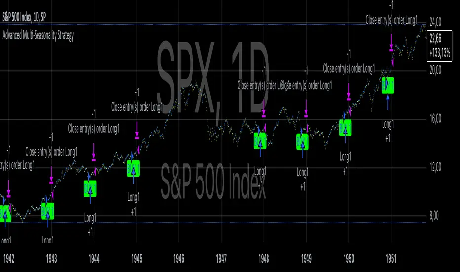
Advanced Multi-Seasonality StrategyThe Multi-Seasonality Strategy is a trading system based on seasonal market patterns. Seasonality refers to recurring market trends driven by predictable calendar-based events. These patterns emerge due to economic cycles, corporate activities (e.g., earnings reports), and investor behavior around specific times of the year. Studies have shown that such effects can influence asset prices over defined periods, leading to opportunities for traders who exploit these patterns (Hirshleifer, 2001; Bouman & Jacobsen, 2002).
How the Strategy Works:
The strategy allows the user to define four distinct periods within a calendar year. For each period, the trader selects:
Entry Date (Month and Day): The date to enter the trade.
Holding Period: The number of trading days to remain in the trade after the entry.
Trade Direction: Whether to take a long or short position during that period.
The system is designed with flexibility, enabling the user to activate or deactivate each of the four periods. The idea is to take advantage of seasonal patterns, such as buying during historically strong periods and selling during weaker ones. A well-known example is the "Sell in May and Go Away" phenomenon, which suggests that stock returns are higher from November to April and weaker from May to October (Bouman & Jacobsen, 2002).
Seasonality in Financial Markets:
Seasonal effects have been documented across different asset classes and markets:
Equities: Stock markets tend to exhibit higher returns during certain months, such as the "January effect," where prices rise after year-end tax-loss selling (Haugen & Lakonishok, 1987).
Commodities: Agricultural commodities often follow seasonal planting and harvesting cycles, which impact supply and demand patterns (Fama & French, 1987).
Forex: Currency pairs may show strength or weakness during specific quarters based on macroeconomic factors, such as fiscal year-end flows or central bank policy decisions.
Scientific Basis:
Research shows that market anomalies like seasonality are linked to behavioral biases and institutional practices. For example, investors may respond to tax incentives at the end of the year, and companies may engage in window dressing (Haugen & Lakonishok, 1987). Additionally, macroeconomic factors, such as monetary policy shifts and holiday trading volumes, can also contribute to predictable seasonal trends (Bouman & Jacobsen, 2002).
Risks of Seasonal Trading:
While the strategy seeks to exploit predictable patterns, there are inherent risks:
Market Changes: Seasonal effects observed in the past may weaken or disappear as market conditions evolve. Increased algorithmic trading, globalization, and policy changes can reduce the reliability of historical patterns (Lo, 2004).
Overfitting: One of the risks in seasonal trading is overfitting the strategy to historical data. A pattern that worked in the past may not necessarily work in the future, especially if it was based on random chance or external factors that no longer apply (Sullivan, Timmermann, & White, 1999).
Liquidity and Volatility: Trading during specific periods may expose the trader to low liquidity, especially around holidays or earnings seasons, leading to slippage and larger-than-expected price swings.
Economic and Geopolitical Shocks: External events such as pandemics, wars, or political instability can disrupt seasonal patterns, leading to unexpected market behavior.
Conclusion:
The Multi-Seasonality Strategy capitalizes on the predictable nature of certain calendar-based patterns in financial markets. By entering and exiting trades based on well-established seasonal effects, traders can potentially capture short-term profits. However, caution is necessary, as market dynamics can change, and seasonal patterns are not guaranteed to persist. Rigorous backtesting, combined with risk management practices, is essential to successfully implementing this strategy.
References:
Bouman, S., & Jacobsen, B. (2002). The Halloween Indicator, "Sell in May and Go Away": Another Puzzle. American Economic Review, 92(5), 1618-1635.
Fama, E. F., & French, K. R. (1987). Commodity Futures Prices: Some Evidence on Forecast Power, Premiums, and the Theory of Storage. Journal of Business, 60(1), 55-73.
Haugen, R. A., & Lakonishok, J. (1987). The Incredible January Effect: The Stock Market's Unsolved Mystery. Dow Jones-Irwin.
Hirshleifer, D. (2001). Investor Psychology and Asset Pricing. Journal of Finance, 56(4), 1533-1597.
Lo, A. W. (2004). The Adaptive Markets Hypothesis: Market Efficiency from an Evolutionary Perspective. Journal of Portfolio Management, 30(5), 15-29.
Sullivan, R., Timmermann, A., & White, H. (1999). Data-Snooping, Technical Trading Rule Performance, and the Bootstrap. Journal of Finance, 54(5), 1647-1691.
This strategy harnesses the power of seasonality but requires careful consideration of the risks and potential changes in market behavior over time.
Statistical ArbitrageThe Statistical Arbitrage Strategy, also known as pairs trading, is a quantitative trading method that capitalizes on price discrepancies between two correlated assets. The strategy assumes that over time, the prices of these two assets will revert to their historical relationship. The core idea is to take advantage of mean reversion, a principle suggesting that asset prices will revert to their long-term average after deviating significantly.
Strategy Mechanics:
1. Selection of Correlated Assets:
• The strategy focuses on two historically correlated assets (e.g., equity index futures like Dow Jones Mini and S&P 500 Mini). These assets tend to move in the same direction due to similar underlying fundamentals, such as overall market conditions. By tracking their relative prices, the strategy seeks to exploit temporary mispricings.
2. Spread Calculation:
• The spread is the difference between the prices of the two assets. This spread represents the relationship between the assets and serves as the basis for determining when to enter or exit trades.
3. Mean and Standard Deviation:
• The historical average (mean) of the spread is calculated using a Simple Moving Average (SMA) over a chosen period. The strategy also computes the standard deviation (volatility) of the spread, which measures how far the spread has deviated from the mean over time. This allows the strategy to define statistically significant price deviations.
4. Entry Signal (Mean Reversion):
• A buy signal is triggered when the spread falls below the mean by a multiple (e.g., two) of the standard deviation. This indicates that one asset is temporarily undervalued relative to the other, and the strategy expects the spread to revert to its mean, generating profits as the prices converge.
5. Exit Signal:
• The strategy exits the trade when the spread reverts to the mean. At this point, the mispricing has been corrected, and the profit from the mean reversion is realized.
Academic Support:
Statistical arbitrage has been widely studied in finance and economics. Gatev, Goetzmann, and Rouwenhorst’s (2006) landmark study on pairs trading demonstrated that this strategy could generate excess returns in equity markets. Their research found that by focusing on historically correlated stocks, traders could identify pricing anomalies and profit from their eventual correction.
Additionally, Avellaneda and Lee (2010) explored statistical arbitrage in different asset classes and found that exploiting deviations in price relationships can offer a robust, market-neutral trading strategy. In these studies, the strategy’s success hinges on the stability of the relationship between the assets and the timely execution of trades when deviations occur.
Risks of Statistical Arbitrage:
1. Correlation Breakdown:
• One of the primary risks is the breakdown of correlation between the two assets. Statistical arbitrage assumes that the historical relationship between the assets will hold in the future. However, market conditions, company fundamentals, or external shocks (e.g., macroeconomic changes) can cause these assets to deviate permanently, leading to potential losses.
• For instance, if two equity indices historically move together but experience divergent economic conditions or policy changes, their prices may no longer revert to the expected mean.
2. Execution Risk:
• This strategy relies on efficient execution and tight spreads. In volatile or illiquid markets, the actual price at which trades are executed may differ significantly from expected prices, leading to slippage and reduced profits.
3. Market Risk:
• Although statistical arbitrage is designed to be market-neutral (i.e., not dependent on the overall market direction), it is not entirely risk-free. Systematic market shocks, such as financial crises or sudden shifts in market sentiment, can affect both assets simultaneously, causing the spread to widen rather than revert to the mean.
4. Model Risk:
• The assumptions underlying the strategy, particularly regarding mean reversion, may not always hold true. The model assumes that asset prices will return to their historical averages within a certain timeframe, but the timing and magnitude of mean reversion can be uncertain. Misestimating this timeframe can lead to extended drawdowns or unrealized losses.
5. Overfitting:
• Over-reliance on historical data to fine-tune the strategy parameters (e.g., the lookback period or standard deviation thresholds) may result in overfitting. This means that the strategy works well on past data but fails to perform in live markets due to changing conditions.
Conclusion:
The Statistical Arbitrage Strategy offers a systematic and quantitative approach to trading that capitalizes on temporary price inefficiencies between correlated assets. It has been proven to generate returns in academic studies and is widely used by hedge funds and institutional traders for its market-neutral characteristics. However, traders must be aware of the inherent risks, including correlation breakdown, execution risks, and the potential for prolonged deviations from the mean. Effective risk management, diversification, and constant monitoring are essential for successfully implementing this strategy in live markets.

ICT Master Suite [Trading IQ]Hello Traders!
We’re excited to introduce the ICT Master Suite by TradingIQ, a new tool designed to bring together several ICT concepts and strategies in one place.
The Purpose Behind the ICT Master Suite
There are a few challenges traders often face when using ICT-related indicators:
Many available indicators focus on one or two ICT methods, which can limit traders who apply a broader range of ICT related techniques on their charts.
There aren't many indicators for ICT strategy models, and we couldn't find ICT indicators that allow for testing the strategy models and setting alerts.
Many ICT related concepts exist in the public domain as indicators, not strategies! This makes it difficult to verify that the ICT concept has some utility in the market you're trading and if it's worth trading - it's difficult to know if it's working!
Some users might not have enough chart space to apply numerous ICT related indicators, which can be restrictive for those wanting to use multiple ICT techniques simultaneously.
The ICT Master Suite is designed to offer a comprehensive option for traders who want to apply a variety of ICT methods. By combining several ICT techniques and strategy models into one indicator, it helps users maximize their chart space while accessing multiple tools in a single slot.
Additionally, the ICT Master Suite was developed as a strategy . This means users can backtest various ICT strategy models - including deep backtesting. A primary goal of this indicator is to let traders decide for themselves what markets to trade ICT concepts in and give them the capability to figure out if the strategy models are worth trading!
What Makes the ICT Master Suite Different
There are many ICT-related indicators available on TradingView, each offering valuable insights. What the ICT Master Suite aims to do is bring together a wider selection of these techniques into one tool. This includes both key ICT methods and strategy models, allowing traders to test and activate strategies all within one indicator.
Features
The ICT Master Suite offers:
Multiple ICT strategy models, including the 2022 Strategy Model and Unicorn Model, which can be built, tested, and used for live trading.
Calculation and display of key price areas like Breaker Blocks, Rejection Blocks, Order Blocks, Fair Value Gaps, Equal Levels, and more.
The ability to set alerts based on these ICT strategies and key price areas.
A comprehensive, yet practical, all-inclusive ICT indicator for traders.
Customizable Timeframe - Calculate ICT concepts on off-chart timeframes
Unicorn Strategy Model
2022 Strategy Model
Liquidity Raid Strategy Model
OTE (Optimal Trade Entry) Strategy Model
Silver Bullet Strategy Model
Order blocks
Breaker blocks
Rejection blocks
FVG
Strong highs and lows
Displacements
Liquidity sweeps
Power of 3
ICT Macros
HTF previous bar high and low
Break of Structure indications
Market Structure Shift indications
Equal highs and lows
Swings highs and swing lows
Fibonacci TPs and SLs
Swing level TPs and SLs
Previous day high and low TPs and SLs
And much more! An ongoing project!
How To Use
Many traders will already be familiar with the ICT related concepts listed above, and will find using the ICT Master Suite quite intuitive!
Despite this, let's go over the features of the tool in-depth and how to use the tool!
The image above shows the ICT Master Suite with almost all techniques activated.
ICT 2022 Strategy Model
The ICT Master suite provides the ability to test, set alerts for, and live trade the ICT 2022 Strategy Model.
The image above shows an example of a long position being entered following a complete setup for the 2022 ICT model.
A liquidity sweep occurs prior to an upside breakout. During the upside breakout the model looks for the FVG that is nearest 50% of the setup range. A limit order is placed at this FVG for entry.
The target entry percentage for the range is customizable in the settings. For instance, you can select to enter at an FVG nearest 33% of the range, 20%, 66%, etc.
The profit target for the model generally uses the highest high of the range (100%) for longs and the lowest low of the range (100%) for shorts. Stop losses are generally set at 0% of the range.
The image above shows the short model in action!
Whether you decide to follow the 2022 model diligently or not, you can still set alerts when the entry condition is met.
ICT Unicorn Model
The image above shows an example of a long position being entered following a complete setup for the ICT Unicorn model.
A lower swing low followed by a higher swing high precedes the overlap of an FVG and breaker block formed during the sequence.
During the upside breakout the model looks for an FVG and breaker block that formed during the sequence and overlap each other. A limit order is placed at the nearest overlap point to current price.
The profit target for this example trade is set at the swing high and the stop loss at the swing low. However, both the profit target and stop loss for this model are configurable in the settings.
For Longs, the selectable profit targets are:
Swing High
Fib -0.5
Fib -1
Fib -2
For Longs, the selectable stop losses are:
Swing Low
Bottom of FVG or breaker block
The image above shows the short version of the Unicorn Model in action!
For Shorts, the selectable profit targets are:
Swing Low
Fib -0.5
Fib -1
Fib -2
For Shorts, the selectable stop losses are:
Swing High
Top of FVG or breaker block
The image above shows the profit target and stop loss options in the settings for the Unicorn Model.
Optimal Trade Entry (OTE) Model
The image above shows an example of a long position being entered following a complete setup for the OTE model.
Price retraces either 0.62, 0.705, or 0.79 of an upside move and a trade is entered.
The profit target for this example trade is set at the -0.5 fib level. This is also adjustable in the settings.
For Longs, the selectable profit targets are:
Swing High
Fib -0.5
Fib -1
Fib -2
The image above shows the short version of the OTE Model in action!
For Shorts, the selectable profit targets are:
Swing Low
Fib -0.5
Fib -1
Fib -2
Liquidity Raid Model
The image above shows an example of a long position being entered following a complete setup for the Liquidity Raid Modell.
The user must define the session in the settings (for this example it is 13:30-16:00 NY time).
During the session, the indicator will calculate the session high and session low. Following a “raid” of either the session high or session low (after the session has completed) the script will look for an entry at a recently formed breaker block.
If the session high is raided the script will look for short entries at a bearish breaker block. If the session low is raided the script will look for long entries at a bullish breaker block.
For Longs, the profit target options are:
Swing high
User inputted Lib level
For Longs, the stop loss options are:
Swing low
User inputted Lib level
Breaker block bottom
The image above shows the short version of the Liquidity Raid Model in action!
For Shorts, the profit target options are:
Swing Low
User inputted Lib level
For Shorts, the stop loss options are:
Swing High
User inputted Lib level
Breaker block top
Silver Bullet Model
The image above shows an example of a long position being entered following a complete setup for the Silver Bullet Modell.
During the session, the indicator will determine the higher timeframe bias. If the higher timeframe bias is bullish the strategy will look to enter long at an FVG that forms during the session. If the higher timeframe bias is bearish the indicator will look to enter short at an FVG that forms during the session.
For Longs, the profit target options are:
Nearest Swing High Above Entry
Previous Day High
For Longs, the stop loss options are:
Nearest Swing Low
Previous Day Low
The image above shows the short version of the Silver Bullet Model in action!
For Shorts, the profit target options are:
Nearest Swing Low Below Entry
Previous Day Low
For Shorts, the stop loss options are:
Nearest Swing High
Previous Day High
Order blocks
The image above shows indicator identifying and labeling order blocks.
The color of the order blocks, and how many should be shown, are configurable in the settings!
Breaker Blocks
The image above shows indicator identifying and labeling order blocks.
The color of the breaker blocks, and how many should be shown, are configurable in the settings!
Rejection Blocks
The image above shows indicator identifying and labeling rejection blocks.
The color of the rejection blocks, and how many should be shown, are configurable in the settings!
Fair Value Gaps
The image above shows indicator identifying and labeling fair value gaps.
The color of the fair value gaps, and how many should be shown, are configurable in the settings!
Additionally, you can select to only show fair values gaps that form after a liquidity sweep. Doing so reduces "noisy" FVGs and focuses on identifying FVGs that form after a significant trading event.
The image above shows the feature enabled. A fair value gap that occurred after a liquidity sweep is shown.
Market Structure
The image above shows the ICT Master Suite calculating market structure shots and break of structures!
The color of MSS and BoS, and whether they should be displayed, are configurable in the settings.
Displacements
The images above show indicator identifying and labeling displacements.
The color of the displacements, and how many should be shown, are configurable in the settings!
Equal Price Points
The image above shows the indicator identifying and labeling equal highs and equal lows.
The color of the equal levels, and how many should be shown, are configurable in the settings!
Previous Custom TF High/Low
The image above shows the ICT Master Suite calculating the high and low price for a user-defined timeframe. In this case the previous day’s high and low are calculated.
To illustrate the customizable timeframe function, the image above shows the indicator calculating the previous 4 hour high and low.
Liquidity Sweeps
The image above shows the indicator identifying a liquidity sweep prior to an upside breakout.
The image above shows the indicator identifying a liquidity sweep prior to a downside breakout.
The color and aggressiveness of liquidity sweep identification are adjustable in the settings!
Power Of Three
The image above shows the indicator calculating Po3 for two user-defined higher timeframes!
Macros
The image above shows the ICT Master Suite identifying the ICT macros!
ICT Macros are only displayable on the 5 minute timeframe or less.
Strategy Performance Table
In addition to a full-fledged TradingView backtest for any of the ICT strategy models the indicator offers, a quick-and-easy strategy table exists for the indicator!
The image above shows the strategy performance table in action.
Keep in mind that, because the ICT Master Suite is a strategy script, you can perform fully automatic backtests, deep backtests, easily add commission and portfolio balance and look at pertinent metrics for the ICT strategies you are testing!
Lite Mode
Traders who want the cleanest chart possible can toggle on “Lite Mode”!
In Lite Mode, any neon or “glow” like effects are removed and key levels are marked as strict border boxes. You can also select to remove box borders if that’s what you prefer!
Settings Used For Backtest
For the displayed backtest, a starting balance of $1000 USD was used. A commission of 0.02%, slippage of 2 ticks, a verify price for limit orders of 2 ticks, and 5% of capital investment per order.
A commission of 0.02% was used due to the backtested asset being a perpetual future contract for a crypto currency. The highest commission (lowest-tier VIP) for maker orders on many exchanges is 0.02%. All entered positions take place as maker orders and so do profit target exits. Stop orders exist as stop-market orders.
A slippage of 2 ticks was used to simulate more realistic stop-market orders. A verify limit order settings of 2 ticks was also used. Even though BTCUSDT.P on Binance is liquid, we just want the backtest to be on the safe side. Additionally, the backtest traded 100+ trades over the period. The higher the sample size the better; however, this example test can serve as a starting point for traders interested in ICT concepts.
Community Assistance And Feedback
Given the complexity and idiosyncratic applications of ICT concepts amongst its proponents, the ICT Master Suite’s built-in strategies and level identification methods might not align with everyone's interpretation.
That said, the best we can do is precisely define ICT strategy rules and concepts to a repeatable process, test, and apply them! Whether or not an ICT strategy is trading precisely how you would trade it, seeing the model in action, taking trades, and with performance statistics is immensely helpful in assessing predictive utility.
If you think we missed something, you notice a bug, have an idea for strategy model improvement, please let us know! The ICT Master Suite is an ongoing project that will, ideally, be shaped by the community.
A big thank you to the @PineCoders for their Time Library!
Thank you!

Williams %R StrategyThe Williams %R Strategy implemented in Pine Script™ is a trading system based on the Williams %R momentum oscillator. The Williams %R indicator, developed by Larry Williams in 1973, is designed to identify overbought and oversold conditions in a market, helping traders time their entries and exits effectively (Williams, 1979). This particular strategy aims to capitalize on short-term price reversals in the S&P 500 (SPY) by identifying extreme values in the Williams %R indicator and using them as trading signals.
Strategy Rules:
Entry Signal:
A long position is entered when the Williams %R value falls below -90, indicating an oversold condition. This threshold suggests that the market may be near a short-term bottom, and prices are likely to reverse or rebound in the short term (Murphy, 1999).
Exit Signal:
The long position is exited when:
The current close price is higher than the previous day’s high, or
The Williams %R indicator rises above -30, indicating that the market is no longer oversold and may be approaching an overbought condition (Wilder, 1978).
Technical Analysis and Rationale:
The Williams %R is a momentum oscillator that measures the level of the close relative to the high-low range over a specific period, providing insight into whether an asset is trading near its highs or lows. The indicator values range from -100 (most oversold) to 0 (most overbought). When the value falls below -90, it indicates an oversold condition where a reversal is likely (Achelis, 2000). This strategy uses this oversold threshold as a signal to initiate long positions, betting on mean reversion—an established principle in financial markets where prices tend to revert to their historical averages (Jegadeesh & Titman, 1993).
Optimization and Performance:
The strategy allows for an adjustable lookback period (between 2 and 25 days) to determine the range used in the Williams %R calculation. Empirical tests show that shorter lookback periods (e.g., 2 days) yield the most favorable outcomes, with profit factors exceeding 2. This finding aligns with studies suggesting that shorter timeframes can effectively capture short-term momentum reversals (Fama, 1970; Jegadeesh & Titman, 1993).
Scientific Context:
Mean Reversion Theory: The strategy’s core relies on mean reversion, which suggests that prices fluctuate around a mean or average value. Research shows that such strategies, particularly those using oscillators like Williams %R, can exploit these temporary deviations (Poterba & Summers, 1988).
Behavioral Finance: The overbought and oversold conditions identified by Williams %R align with psychological factors influencing trading behavior, such as herding and panic selling, which often create opportunities for price reversals (Shiller, 2003).
Conclusion:
This Williams %R-based strategy utilizes a well-established momentum oscillator to time entries and exits in the S&P 500. By targeting extreme oversold conditions and exiting when these conditions revert or exceed historical ranges, the strategy aims to capture short-term gains. Scientific evidence supports the effectiveness of short-term mean reversion strategies, particularly when using indicators sensitive to momentum shifts.
References:
Achelis, S. B. (2000). Technical Analysis from A to Z. McGraw Hill.
Fama, E. F. (1970). Efficient Capital Markets: A Review of Theory and Empirical Work. The Journal of Finance, 25(2), 383-417.
Jegadeesh, N., & Titman, S. (1993). Returns to Buying Winners and Selling Losers: Implications for Stock Market Efficiency. The Journal of Finance, 48(1), 65-91.
Murphy, J. J. (1999). Technical Analysis of the Financial Markets: A Comprehensive Guide to Trading Methods and Applications. New York Institute of Finance.
Poterba, J. M., & Summers, L. H. (1988). Mean Reversion in Stock Prices: Evidence and Implications. Journal of Financial Economics, 22(1), 27-59.
Shiller, R. J. (2003). From Efficient Markets Theory to Behavioral Finance. Journal of Economic Perspectives, 17(1), 83-104.
Williams, L. (1979). How I Made One Million Dollars… Last Year… Trading Commodities. Windsor Books.
Wilder, J. W. (1978). New Concepts in Technical Trading Systems. Trend Research.
This explanation provides a scientific and evidence-based perspective on the Williams %R trading strategy, aligning it with fundamental principles in technical analysis and behavioral finance.

Indicator Test with Conditions TableOverview: The "Indicator Test with Conditions Table" is a customizable trading strategy developed using Pine Script™ for the TradingView platform. It allows users to define complex entry conditions for both long and short positions based on various technical indicators and price levels.
Key Features:
Customizable Input Conditions:
Users can configure up to three input conditions for both long and short entries, each with its own logical operator (AND/OR) for combining conditions.
Input conditions can be based on:
Price Sources: Users can select any price data (e.g., close, open, high, low) for each condition.
Comparison Operators: Users can choose from a variety of operators, including:
Greater than (>)
Greater than or equal to (>=)
Less than (<)
Less than or equal to (<=)
Equal to (=)
Not equal to (!=)
Crossover (crossover)
Crossunder (crossunder)
Logical Operators:
The strategy provides options for combining conditions using logical operators (AND/OR) for greater flexibility in defining entry criteria.
Dynamic Condition Evaluation:
The strategy evaluates the defined conditions dynamically, checking whether they are enabled before proceeding with the comparison.
Users can toggle conditions on and off using boolean inputs, allowing for quick adjustments without modifying the code.
Visual Feedback:
A table is displayed on the chart, providing real-time status updates on the conditions and whether they are enabled. This enhances user experience by allowing easy monitoring of the strategy's logic.
Order Execution:
The strategy enters long or short positions based on the combined conditions' evaluations, automatically executing trades when the criteria are met.
How to Use:
Set Up Input Conditions:
Navigate to the strategy’s input settings to configure your desired price sources, operators, and logical combinations for long and short conditions.
Monitor Conditions:
Observe the condition table displayed at the bottom right of the chart to see which conditions are enabled and their current evaluations.
Adjust Strategy Parameters:
Modify the conditions, logical operators, and input sources as needed to optimize the strategy for different market scenarios or trading styles.
Execution:
Once the conditions are met, the strategy will automatically enter trades based on the defined logic.
Conclusion: The "Indicator Test with Conditions Table" strategy is a robust tool for traders looking to implement customized trading logic based on various market conditions. Its flexibility and real-time monitoring capabilities make it suitable for both novice and experienced traders.

Monthly Breakout StrategyThis Monthly High/Low Breakout Strategy is designed to take long or short positions based on breakouts from the high or low of the previous month. Users can select whether they want to go long at a breakout above the previous month’s high, short at a breakdown below the previous month’s low, or use the reverse logic. Additionally, it includes a month filter, allowing trades to be executed only during user-specified months.
Breakout strategies, particularly those based on monthly highs and lows, aim to capitalize on price momentum. These systems rely on the assumption that once a significant price level is breached (such as the previous month's high or low), the market is likely to continue moving in the same direction due to increased volatility and trend-following behaviors by traders. Studies have demonstrated the potential effectiveness of breakout strategies in financial markets.
Scientific Evidence Supporting Breakout Strategies:
Momentum in Financial Markets:
Research on momentum-based strategies, which include breakout trading, shows that securities breaking key levels of support or resistance tend to continue their price movement in the direction of the breakout. Jegadeesh and Titman (1993) found that stocks with strong performance over a given period tend to continue performing well in subsequent periods, a principle also applied to breakout strategies.
Behavioral Finance:
The psychological factor of herd behavior is one of the driving forces behind breakout strategies. When prices break out of a key level (such as a monthly high), it triggers increased buying or selling pressure as traders join the trend. Barberis, Shleifer, and Vishny (1998) explained how cognitive biases, such as overconfidence and sentiment, can amplify price trends, which breakout strategies attempt to exploit.
Market Efficiency:
While markets are generally efficient, periods of inefficiency can occur, particularly around the breakouts of significant price levels. These inefficiencies often result in temporary price trends, which breakout strategies can exploit before the market corrects itself (Fama, 1970).
Risk Considerations:
Despite the potential for profit, the Monthly Breakout Strategy comes with several risks:
False Breakouts:
One of the most common risks in breakout strategies is the occurrence of false breakouts. These happen when the price temporarily moves above (or below) a key level but quickly reverses direction, causing losses for traders who entered positions too early. This is particularly risky in low-volatility environments.
Market Volatility:
Monthly breakout strategies rely on momentum, which may not be consistent across different market conditions. During periods of low volatility, price breakouts might lack the follow-through required for the strategy to succeed, leading to poor performance.
Whipsaw Risk:
The strategy is vulnerable to whipsaw markets, where prices oscillate around key levels without establishing a clear direction. This can result in frequent entry and exit signals that lead to losses, especially if trading costs are not managed properly.
Overfitting to Past Data:
If the month-selection filter is overly optimized based on historical data, the strategy may suffer from overfitting—performing well in backtests but poorly in real-time trading. This happens when strategies are tailored to past market conditions that may not repeat.
Conclusion:
While monthly breakout strategies can be effective in markets with strong momentum, they are subject to several risks, including false breakouts, volatility dependency, and whipsaw behavior. It is crucial to backtest this strategy thoroughly and ensure it aligns with your risk tolerance before implementing it in live trading.
References:
Jegadeesh, N., & Titman, S. (1993). Returns to Buying Winners and Selling Losers: Implications for Stock Market Efficiency. Journal of Finance, 48(1), 65-91.
Barberis, N., Shleifer, A., & Vishny, R. (1998). A Model of Investor Sentiment. Journal of Financial Economics, 49(3), 307-343.
Fama, E. F. (1970). Efficient Capital Markets: A Review of Theory and Empirical Work. Journal of Finance, 25(2), 383-417.
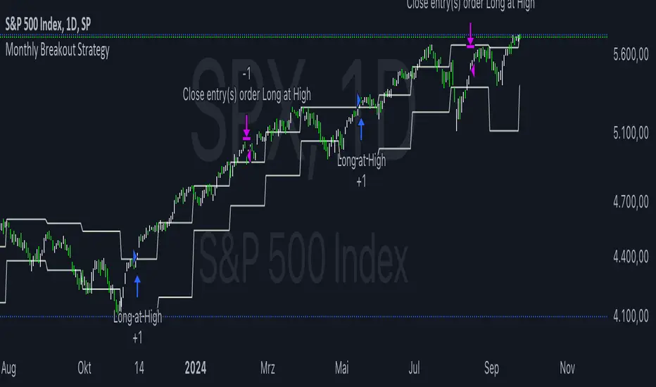
High/Low Breakout Statistical Analysis StrategyThis Pine Script strategy is designed to assist in the statistical analysis of breakout systems on a monthly, weekly, or daily timeframe. It allows the user to select whether to open a long or short position when the price breaks above or below the respective high or low for the chosen timeframe. The user can also define the holding period for each position in terms of bars.
Core Functionality:
Breakout Logic:
The strategy triggers trades based on price crossing over (for long positions) or crossing under (for short positions) the high or low of the selected period (daily, weekly, or monthly).
Timeframe Selection:
A dropdown menu enables the user to switch between the desired timeframe (monthly, weekly, or daily).
Trade Direction:
Another dropdown allows the user to select the type of trade (long or short) depending on whether the breakout occurs at the high or low of the timeframe.
Holding Period:
Once a trade is opened, it is automatically closed after a user-defined number of bars, making it useful for analyzing how breakout signals perform over short-term periods.
This strategy is intended exclusively for research and statistical purposes rather than real-time trading, helping users to assess the behavior of breakouts over different timeframes.
Relevance of Breakout Systems:
Breakout trading systems, where trades are executed when the price moves beyond a significant price level such as the high or low of a given period, have been extensively studied in financial literature for their potential predictive power.
Momentum and Trend Following:
Breakout strategies are a form of momentum-based trading, exploiting the tendency of prices to continue moving in the direction of a strong initial movement after breaching a critical support or resistance level. According to academic research, momentum strategies, including breakouts, can produce returns above average market returns when applied consistently. For example, Jegadeesh and Titman (1993) demonstrated that stocks that performed well in the past 3-12 months continued to outperform in the subsequent months, suggesting that price continuation patterns, like breakouts, hold value .
Market Efficiency Hypothesis:
While the Efficient Market Hypothesis (EMH) posits that markets are generally efficient, and it is difficult to outperform the market through technical strategies, some studies show that in less liquid markets or during specific times of market stress, breakout systems can capitalize on temporary inefficiencies. Taylor (2005) and other researchers have found instances where breakout systems can outperform the market under certain conditions.
Volatility and Breakouts:
Breakouts are often linked to periods of increased volatility, which can generate trading opportunities. Coval and Shumway (2001) found that periods of heightened volatility can make breakouts more significant, increasing the likelihood that price trends will follow the breakout direction. This correlation between volatility and breakout reliability makes it essential to study breakouts across different timeframes to assess their potential profitability .
In summary, this breakout strategy offers an empirical way to study price behavior around key support and resistance levels. It is useful for researchers and traders aiming to statistically evaluate the effectiveness and consistency of breakout signals across different timeframes, contributing to broader research on momentum and market behavior.
References:
Jegadeesh, N., & Titman, S. (1993). Returns to Buying Winners and Selling Losers: Implications for Stock Market Efficiency. Journal of Finance, 48(1), 65-91.
Fama, E. F., & French, K. R. (1996). Multifactor Explanations of Asset Pricing Anomalies. Journal of Finance, 51(1), 55-84.
Taylor, S. J. (2005). Asset Price Dynamics, Volatility, and Prediction. Princeton University Press.
Coval, J. D., & Shumway, T. (2001). Expected Option Returns. Journal of Finance, 56(3), 983-1009.
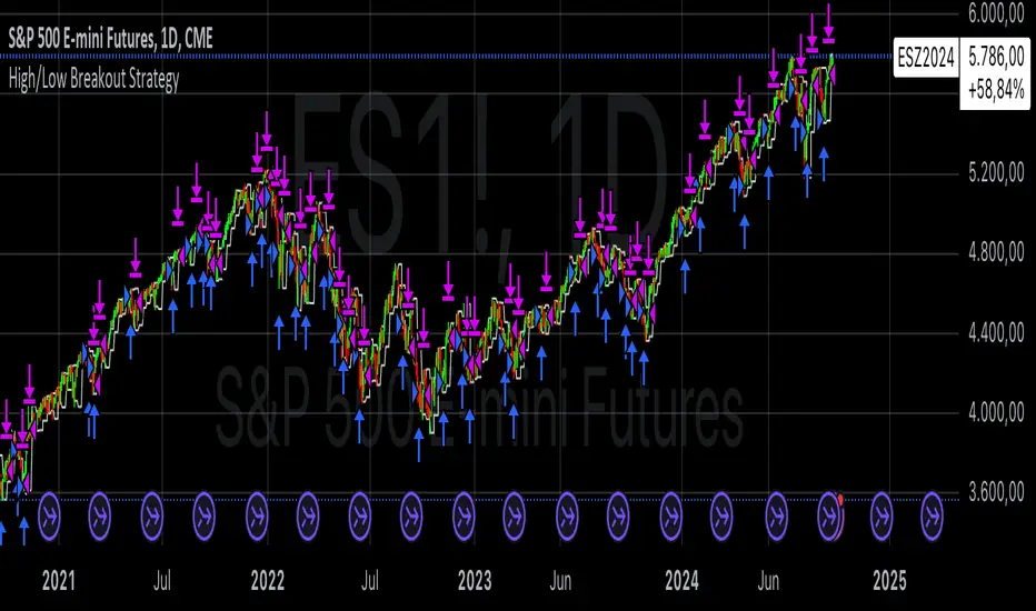
High Yield Spread Strategy with SMA FilterThis Pine Script strategy is designed for statistical analysis and research purposes only, not for live trading or financial decision-making. The script evaluates the relationship between financial volatility (measured by either the VIX or the High Yield Spread) and market positioning strategies (long or short) based on user-defined conditions. Specifically, it allows users to test the assumption that elevated levels of VIX or the High Yield Spread may justify short positions in the market—a widely held belief in financial circles—but this script demonstrates that shorting is not always the optimal choice, even under these conditions.
Key Components:
1. High Yield Spread and VIX:
• High Yield Spread is the difference between the yields of corporate high-yield (or “junk”) bonds and U.S. Treasury securities. A rising spread often reflects increased market risk perception.
• VIX (Volatility Index) is often referred to as the market’s “fear gauge.” Higher VIX levels usually indicate heightened market uncertainty or expected volatility.
2. Strategy Logic:
• The script allows users to specify a threshold for the VIX or High Yield Spread, and it automatically evaluates if the spread exceeds this level, which traditionally would suggest an environment for higher market risk and thus potentially favoring short trades.
• However, the strategy provides flexibility to enter long or short positions, even in a high-risk environment, emphasizing that a high VIX or High Yield Spread does not always warrant shorting.
3. SMA Filter:
• A Simple Moving Average (SMA) filter can be applied to the price data, where positions are only entered if the price is above or below the SMA (depending on the trade direction). This adds a technical component to the strategy, incorporating price trends into decision-making.
4. Hold Duration:
• The script also allows users to define how long to hold a position after entering, enabling an analysis of different timeframes.
Theoretical Background:
The traditional belief that high VIX or High Yield Spreads favor short positions is not universally supported by research. While a spike in the VIX or credit spreads is often associated with increased market risk, research suggests that excessive volatility does not always lead to negative returns. In fact, high volatility can sometimes signal an approaching market rebound.
For example:
• Studies have shown that long-term investments during periods of heightened volatility can yield favorable returns due to mean reversion. Whaley (2000) notes that VIX spikes are often followed by market recoveries as volatility tends to revert to its mean over time .
• Research by Blitz and Vliet (2007) highlights that low-volatility stocks have historically outperformed high-volatility stocks, suggesting that volatility may not always predict negative returns .
• Furthermore, credit spreads can widen in response to broader market stress, but these may overshoot the actual credit risk, presenting opportunities for long positions when spreads are high and risk premiums are mispriced .
Educational Purpose:
The goal of this script is to challenge assumptions about shorting during volatile periods, showing that long positions can be equally, if not more, effective during market stress. By incorporating an SMA filter and customizable logic for entering trades, users can test different hypotheses regarding the effectiveness of both long and short positions under varying market conditions.
Note: This strategy is not intended for live trading and should be used solely for educational and statistical exploration. Misinterpreting financial indicators can lead to incorrect investment decisions, and it is crucial to conduct comprehensive research before trading.
References:
1. Whaley, R. E. (2000). “The Investor Fear Gauge”. The Journal of Portfolio Management, 26(3), 12-17.
2. Blitz, D., & van Vliet, P. (2007). “The Volatility Effect: Lower Risk Without Lower Return”. Journal of Portfolio Management, 34(1), 102-113.
3. Bhamra, H. S., & Kuehn, L. A. (2010). “The Determinants of Credit Spreads: An Empirical Analysis”. Journal of Finance, 65(3), 1041-1072.
This explanation highlights the academic and research-backed foundation of the strategy and the nuances of volatility, while cautioning against the assumption that high VIX or High Yield Spread always calls for shorting.